Formulas you can watch

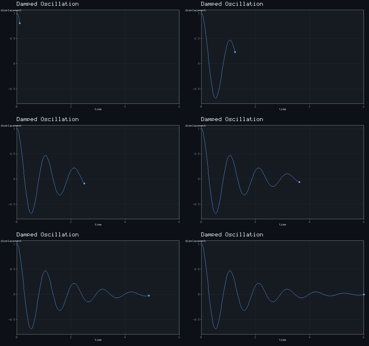
Damped Oscillation

x = A e^(-ζωt) cos(ω_d t)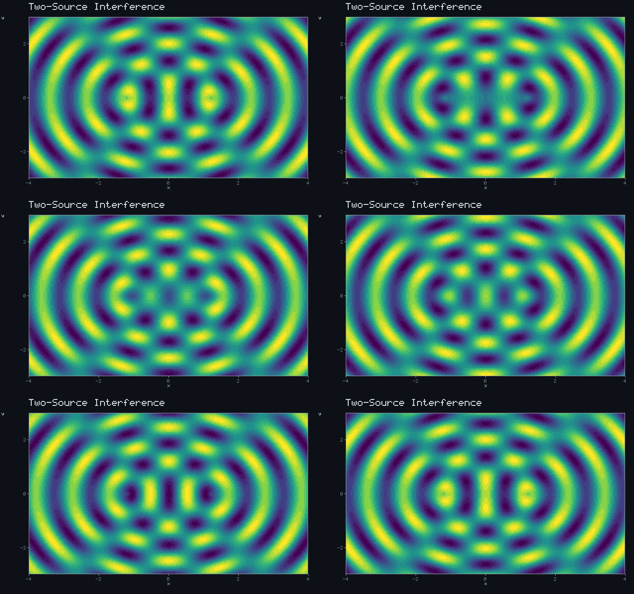

Two-Source Interference

A = sin(k r₁ - ωt) + sin(k r₂ - ωt)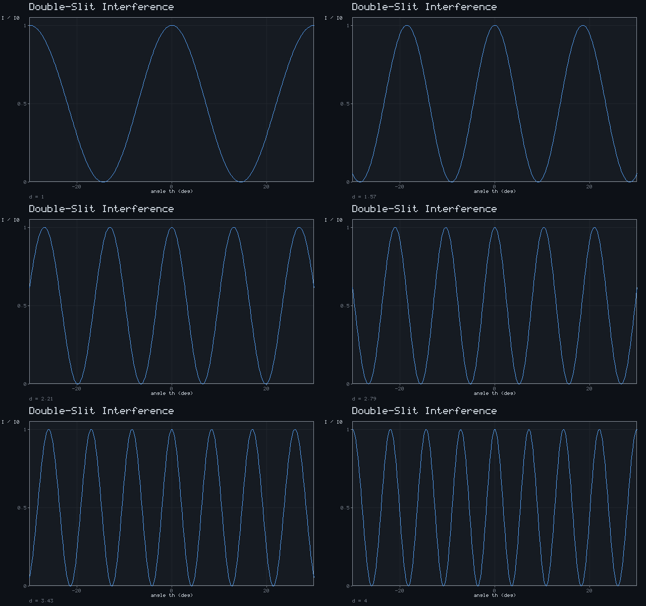

Double-Slit Interference

I = I₀ cos²(π d sinθ / λ)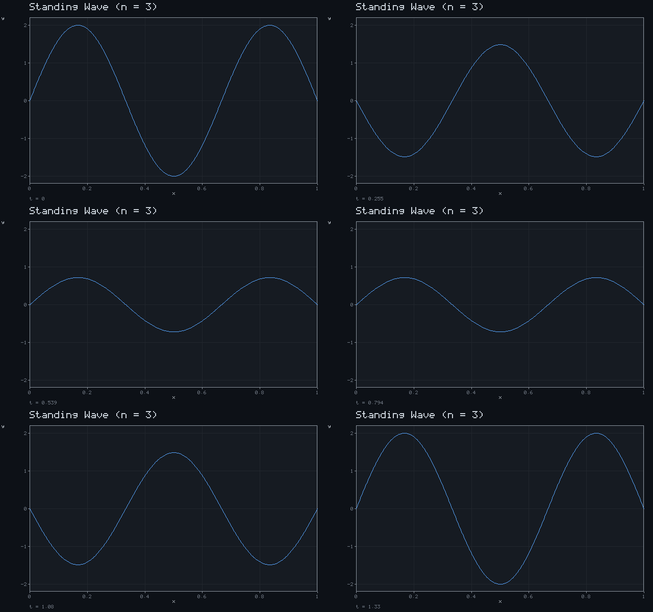

Standing Wave (n = 3)

y = 2A sin(nπx/L) cos(nπvt/L)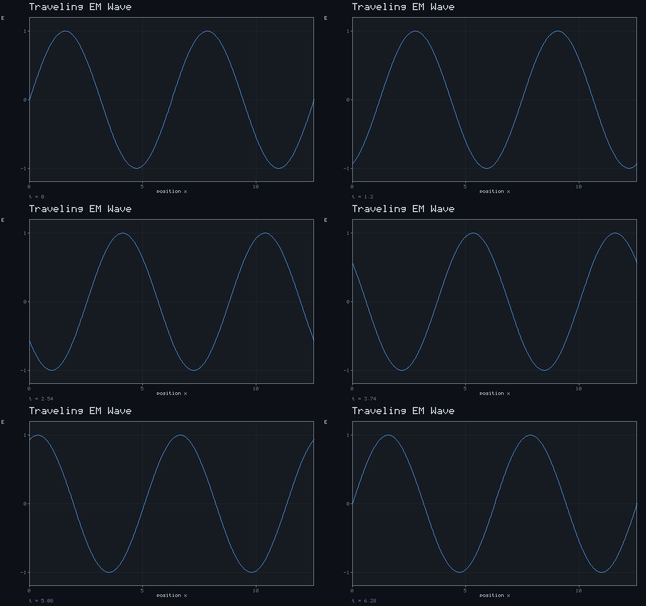

Traveling EM Wave

E = sin(kx − ωt)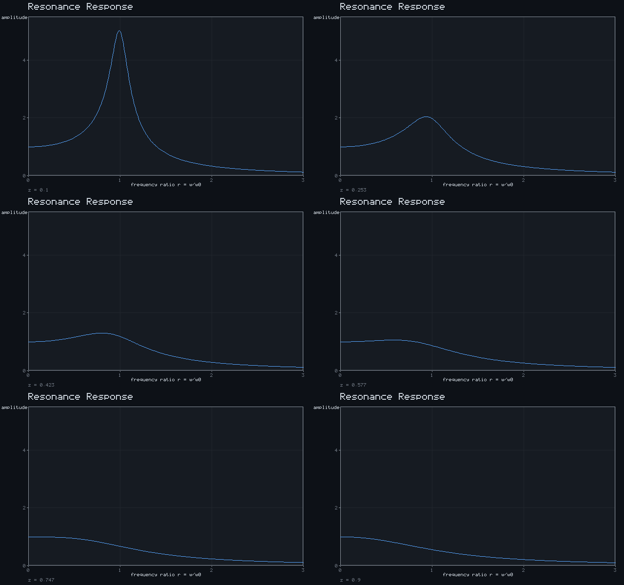

Resonance Response

A = 1/√((1−r²)² + (2ζr)²)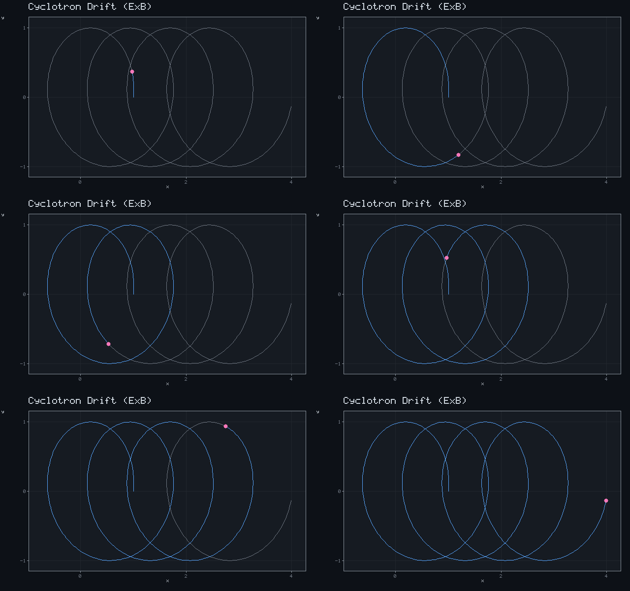

Cyclotron Drift (E×B)

r(t) = (cos ωt + v_d t, sin ωt)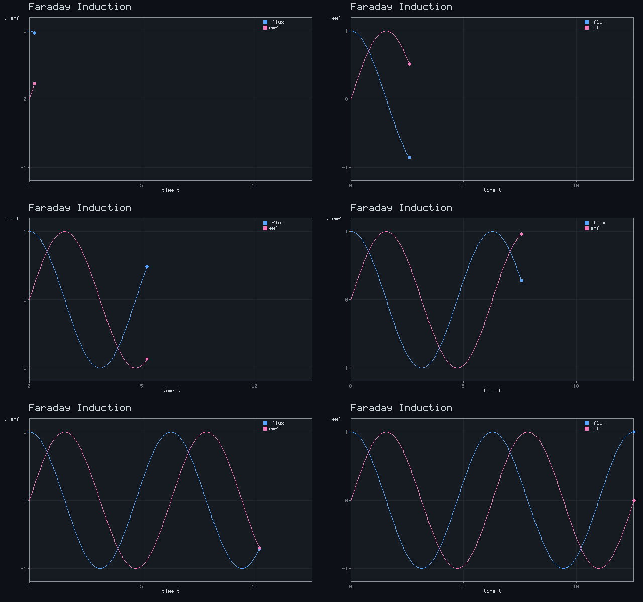

Faraday Induction

emf = −dΦ/dt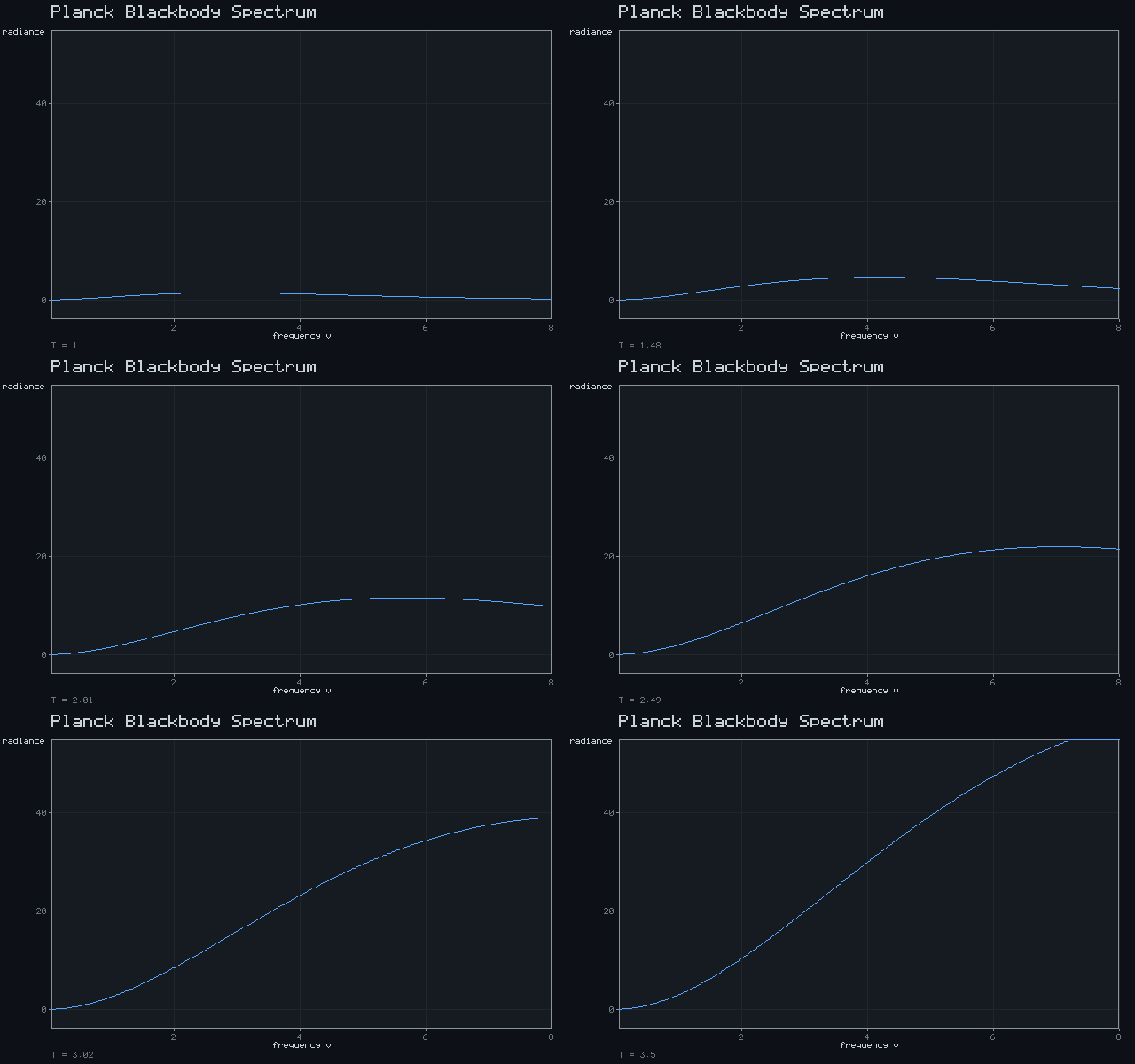

Planck Blackbody Spectrum

B ∝ ν³ / (e^{ν/T} − 1)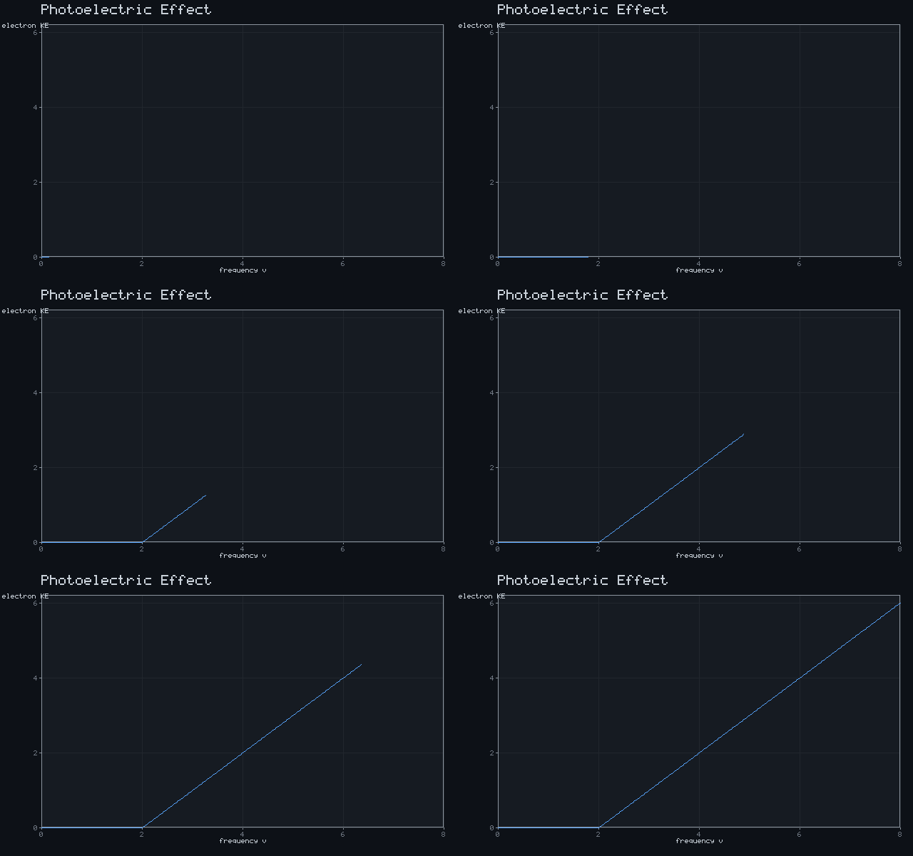

Photoelectric Effect

KE = max(0, hν − φ)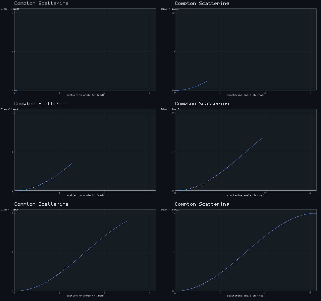

Compton Scattering

Δλ = λ_C (1 − cosθ)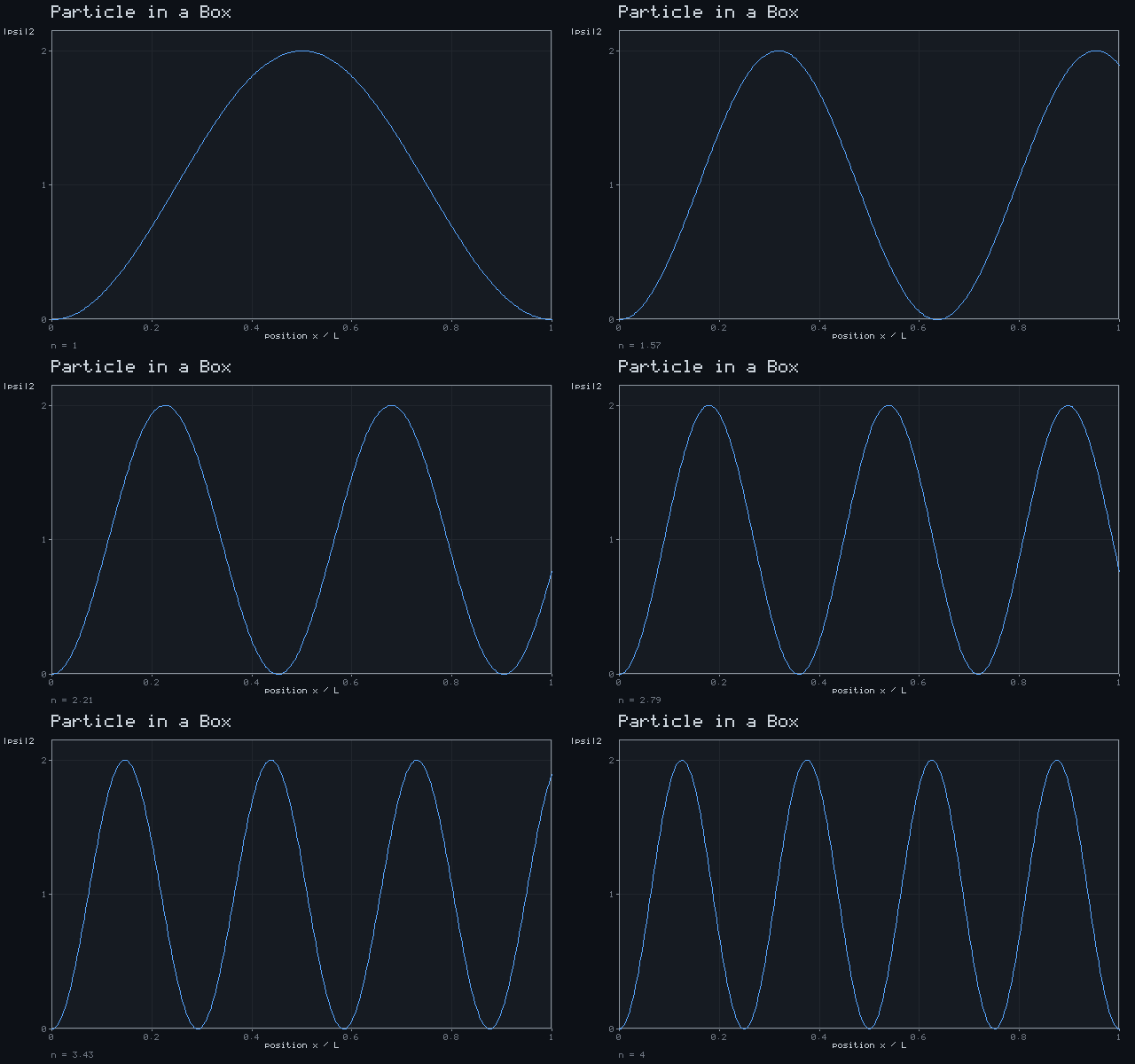

Particle in a Box

|ψ|² = 2 sin²(nπx)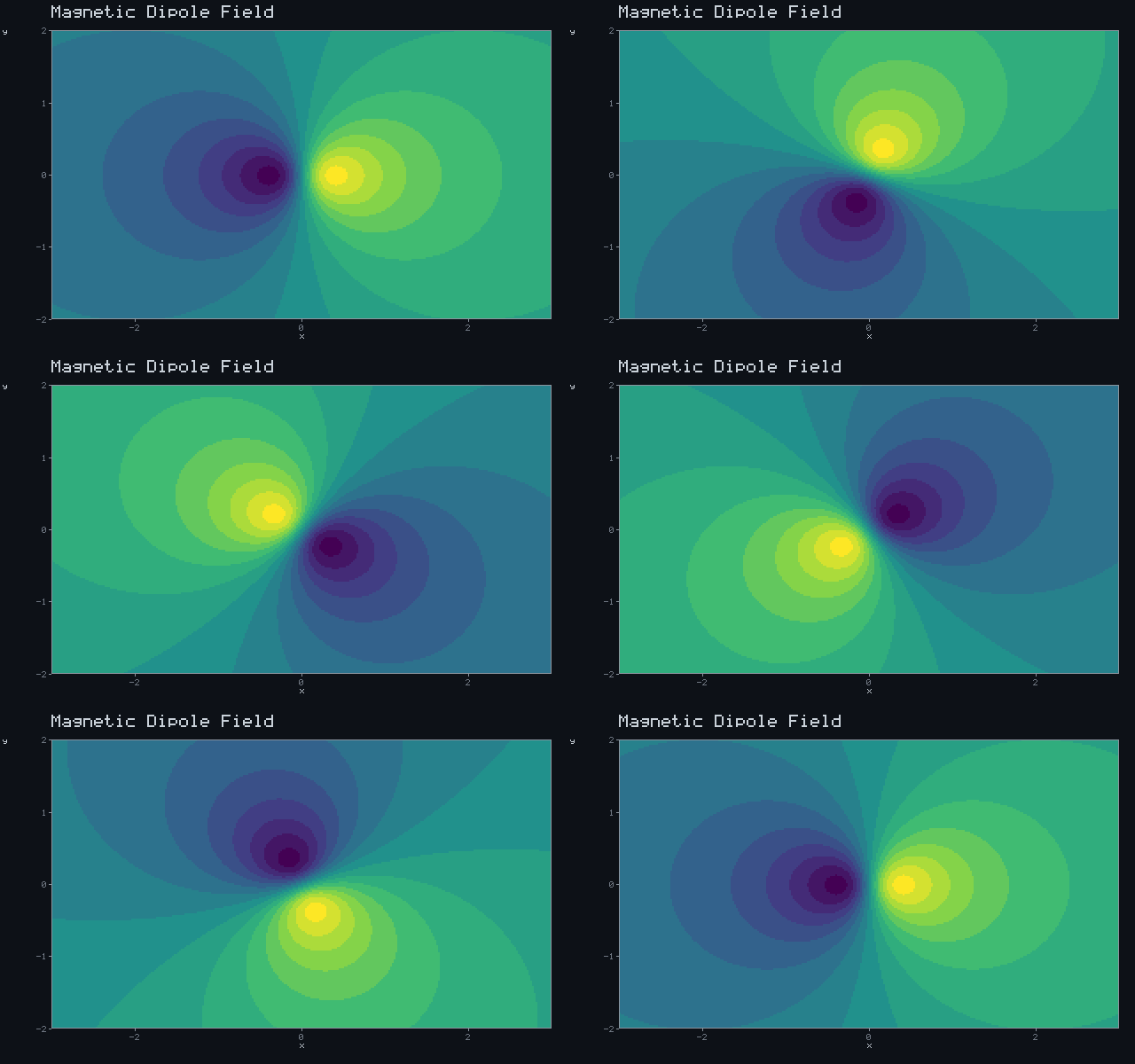

Magnetic Dipole Field

Φ ∝ cosθ / r²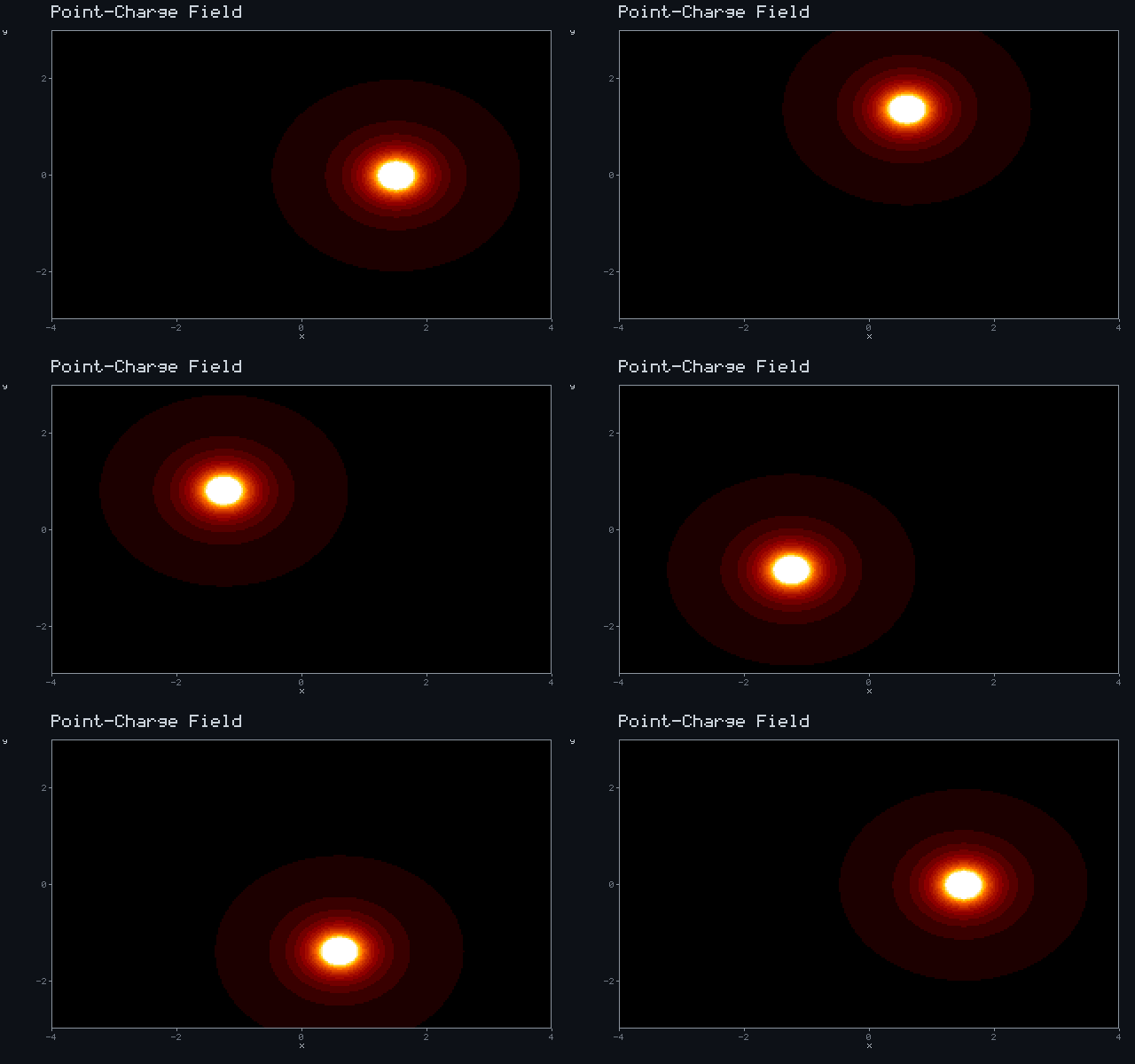

Point-Charge Field

|E| ∝ 1 / r²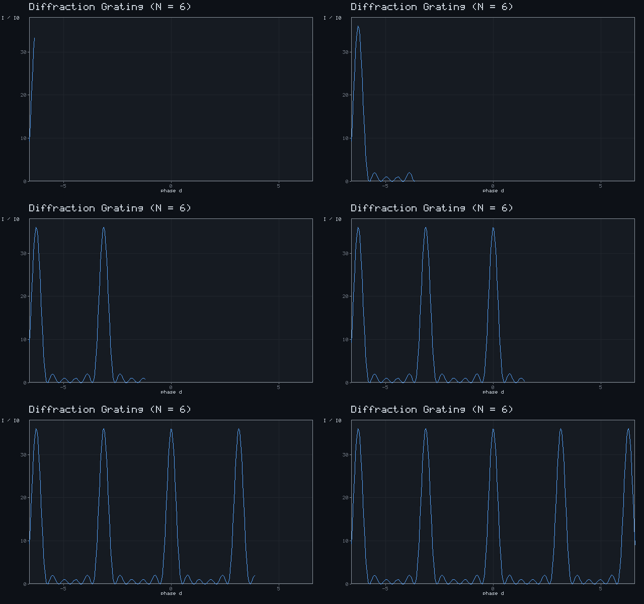

Diffraction Grating (N = 6)

I = (sin Nδ / sin δ)²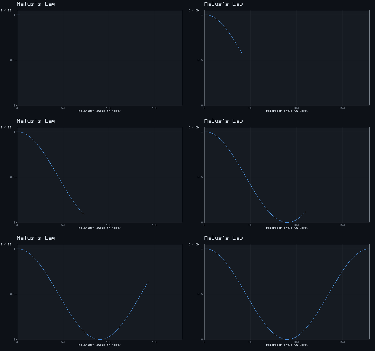

Malus's Law

I = I₀ cos²θ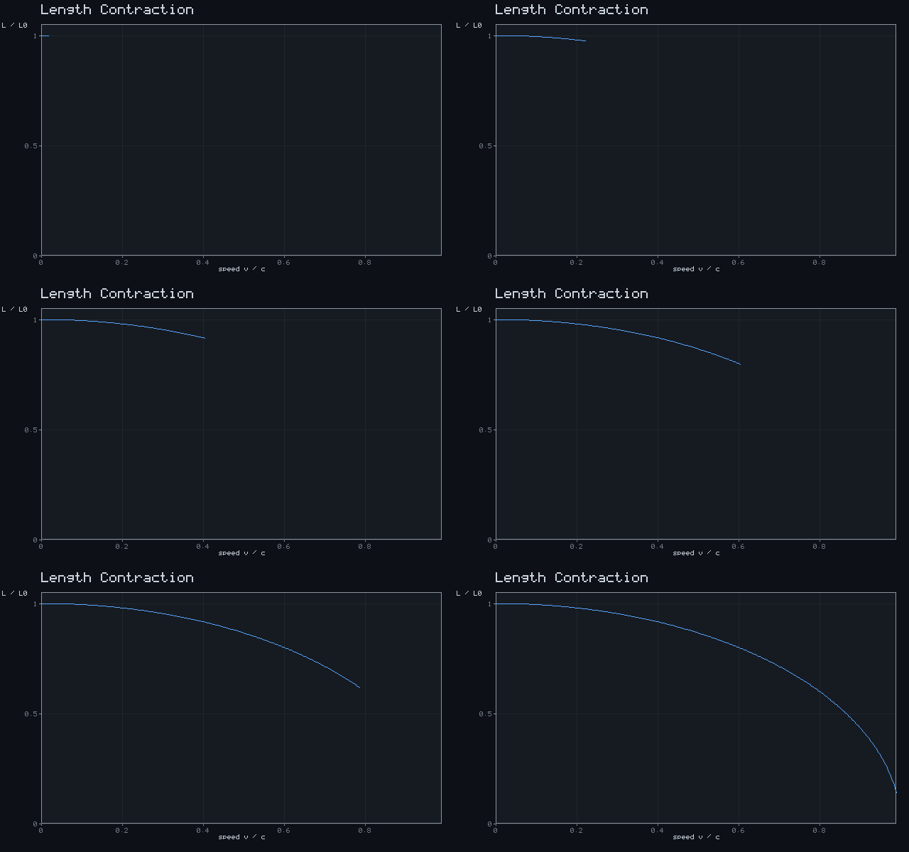

Length Contraction

L = L₀ √(1 − v²/c²)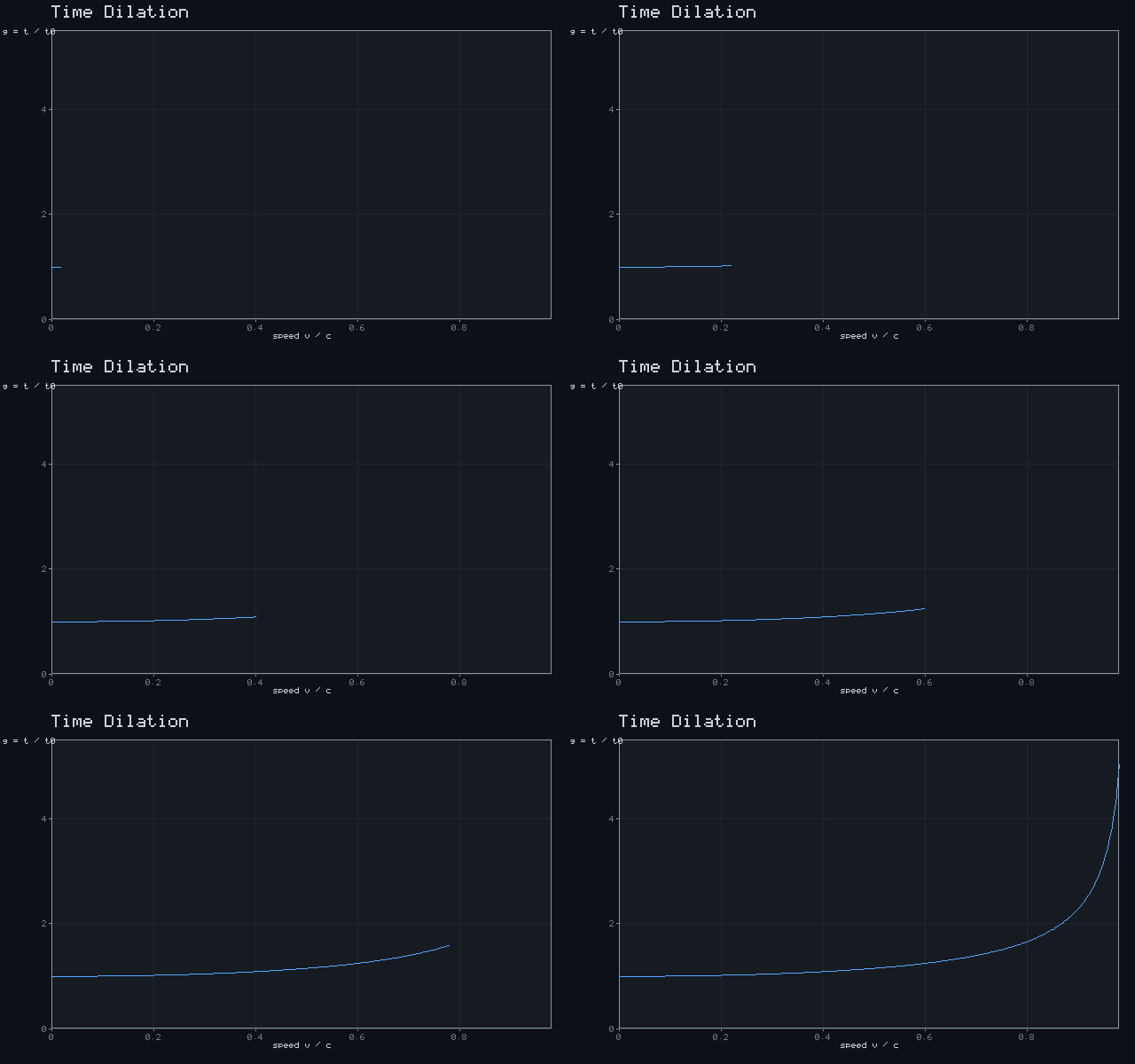

Time Dilation

t = t₀ / √(1 − v²/c²)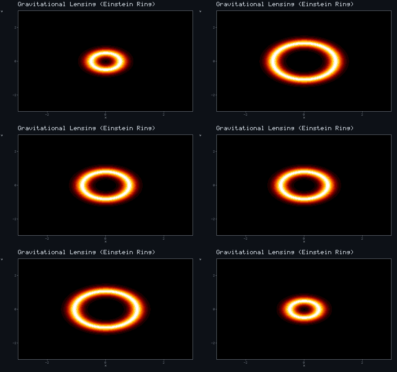

Gravitational Lensing (Einstein Ring)

α = 4GM / (c²b)

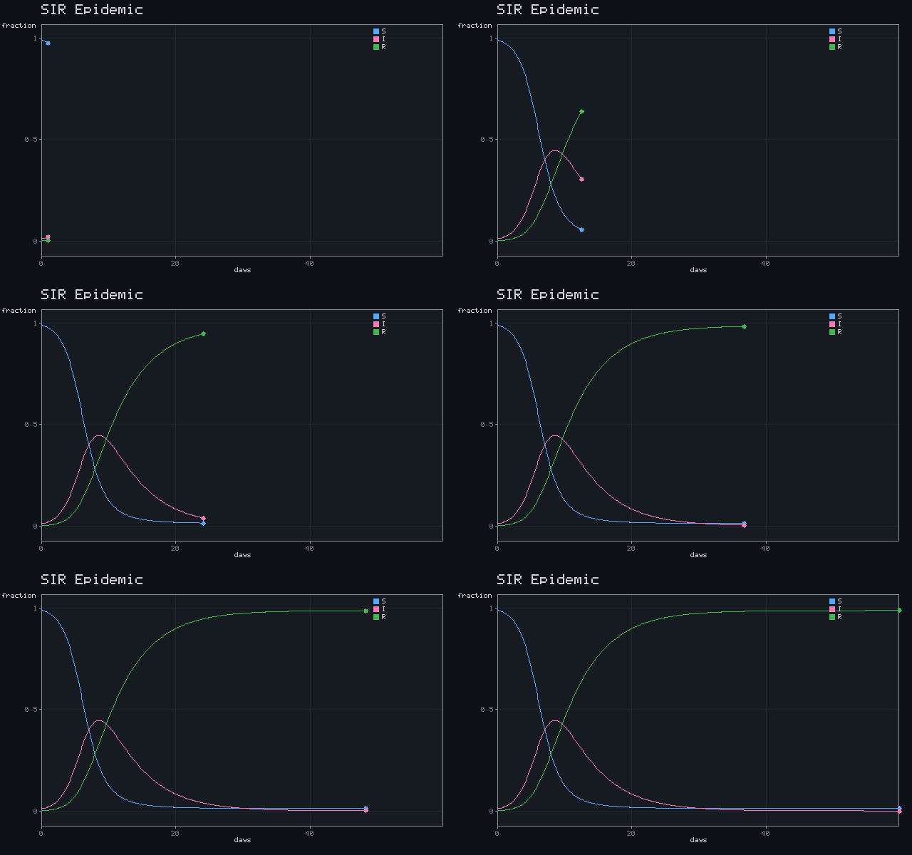
SIR Epidemic

S'=-βSI · I'=βSI-γI · R'=γI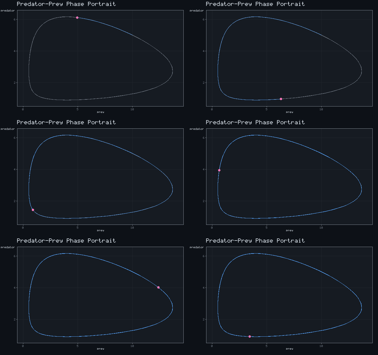

Predator-Prey Phase Portrait

N'=αN-βNP · P'=δNP-γP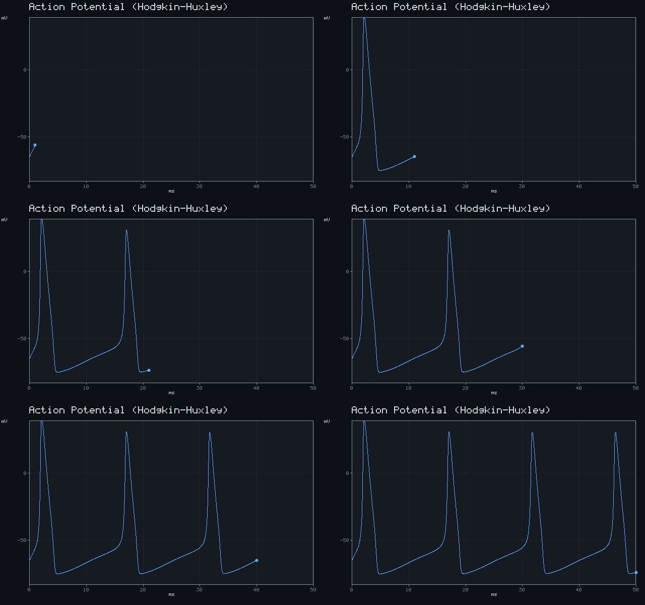

Action Potential (Hodgkin-Huxley)

C dV/dt = I − gNa·m³h(V−ENa) − gK·n⁴(V−EK) − gL(V−EL)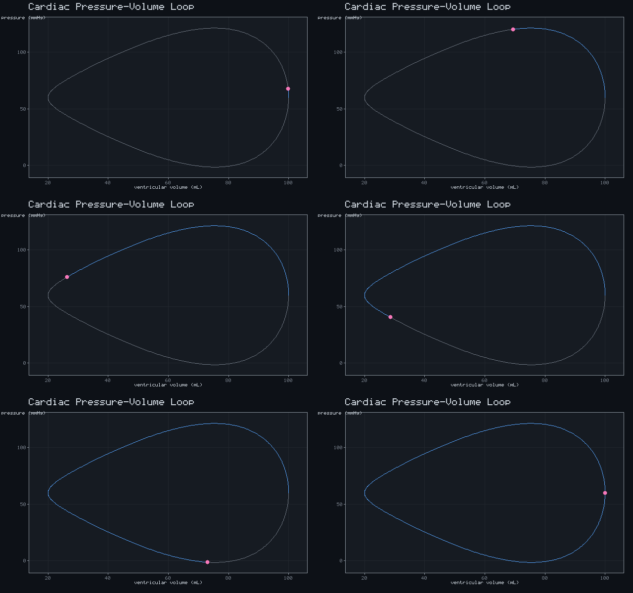

Cardiac Pressure-Volume Loop

counter-clockwise P-V trajectory of one heartbeat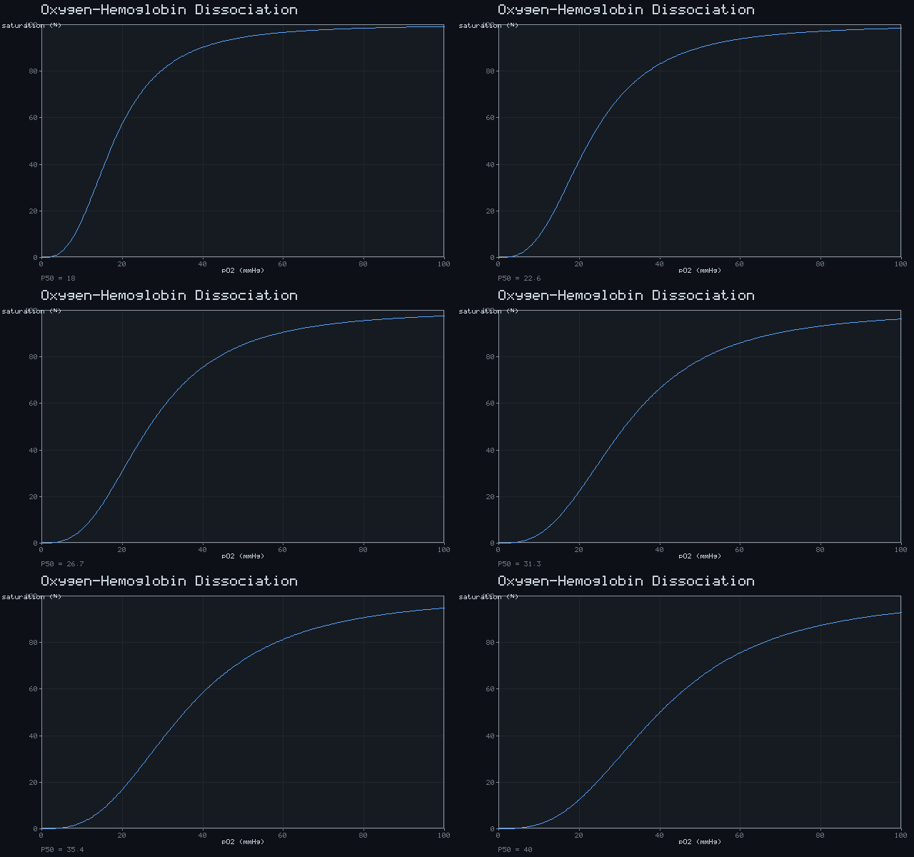

Oxygen-Hemoglobin Dissociation

S = pO₂ⁿ / (pO₂ⁿ + P50ⁿ), n ≈ 2.8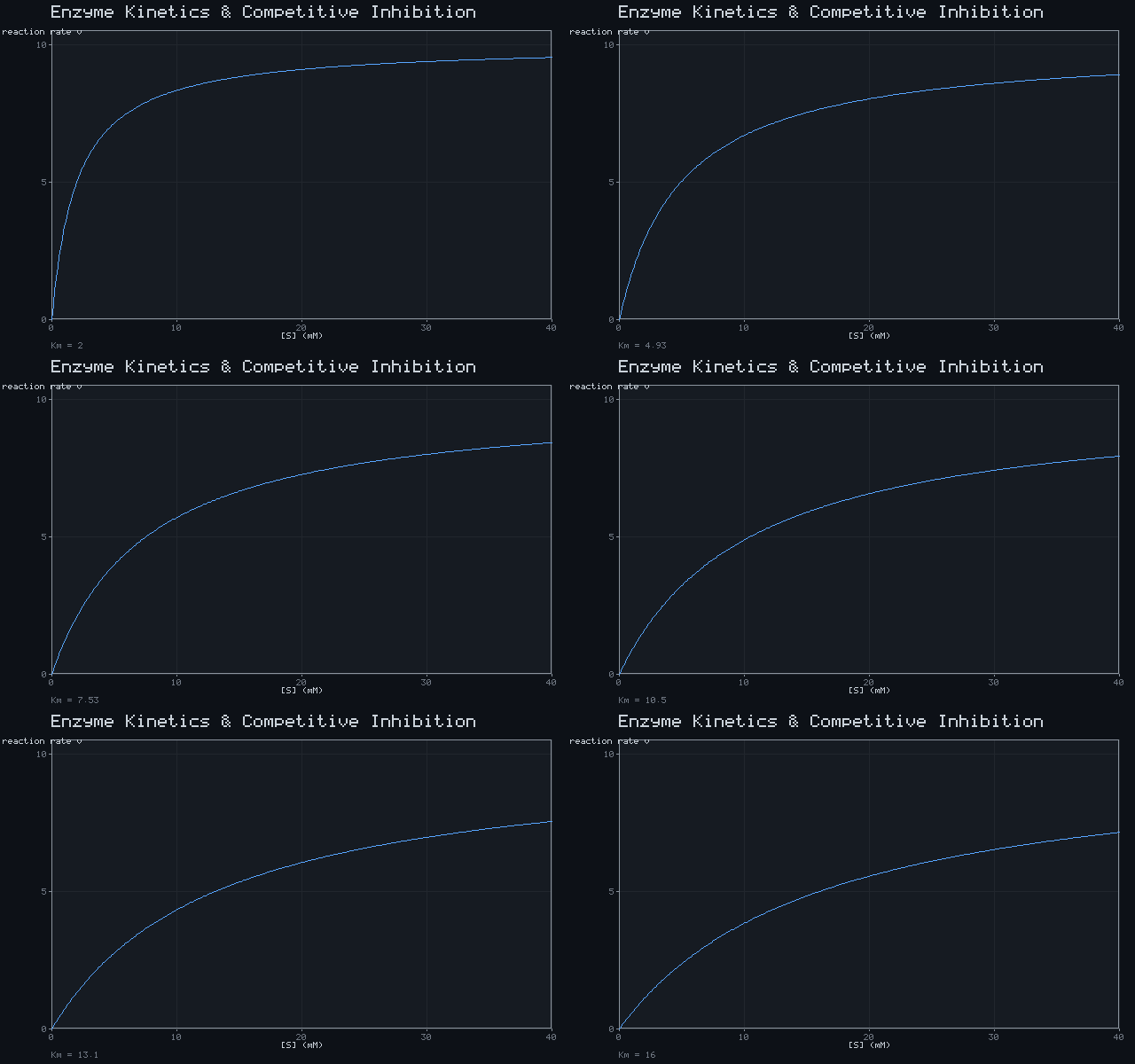

Enzyme Kinetics & Competitive Inhibition

v = Vmax·[S] / (Km + [S])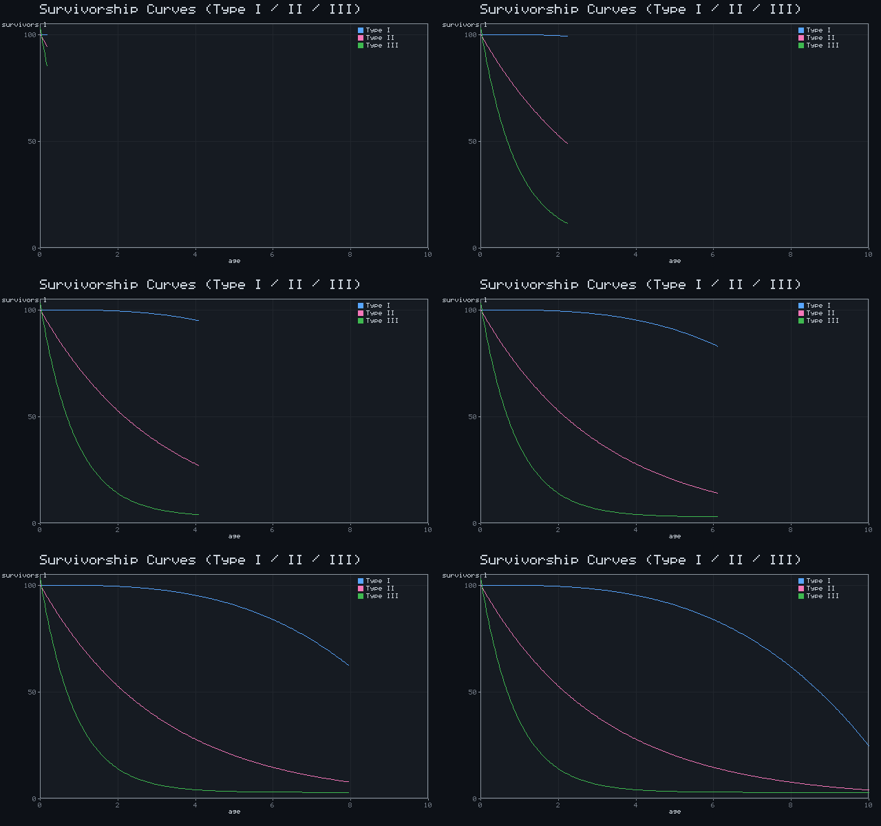

Survivorship Curves (Type I / II / III)

lₓ = survivors as a function of age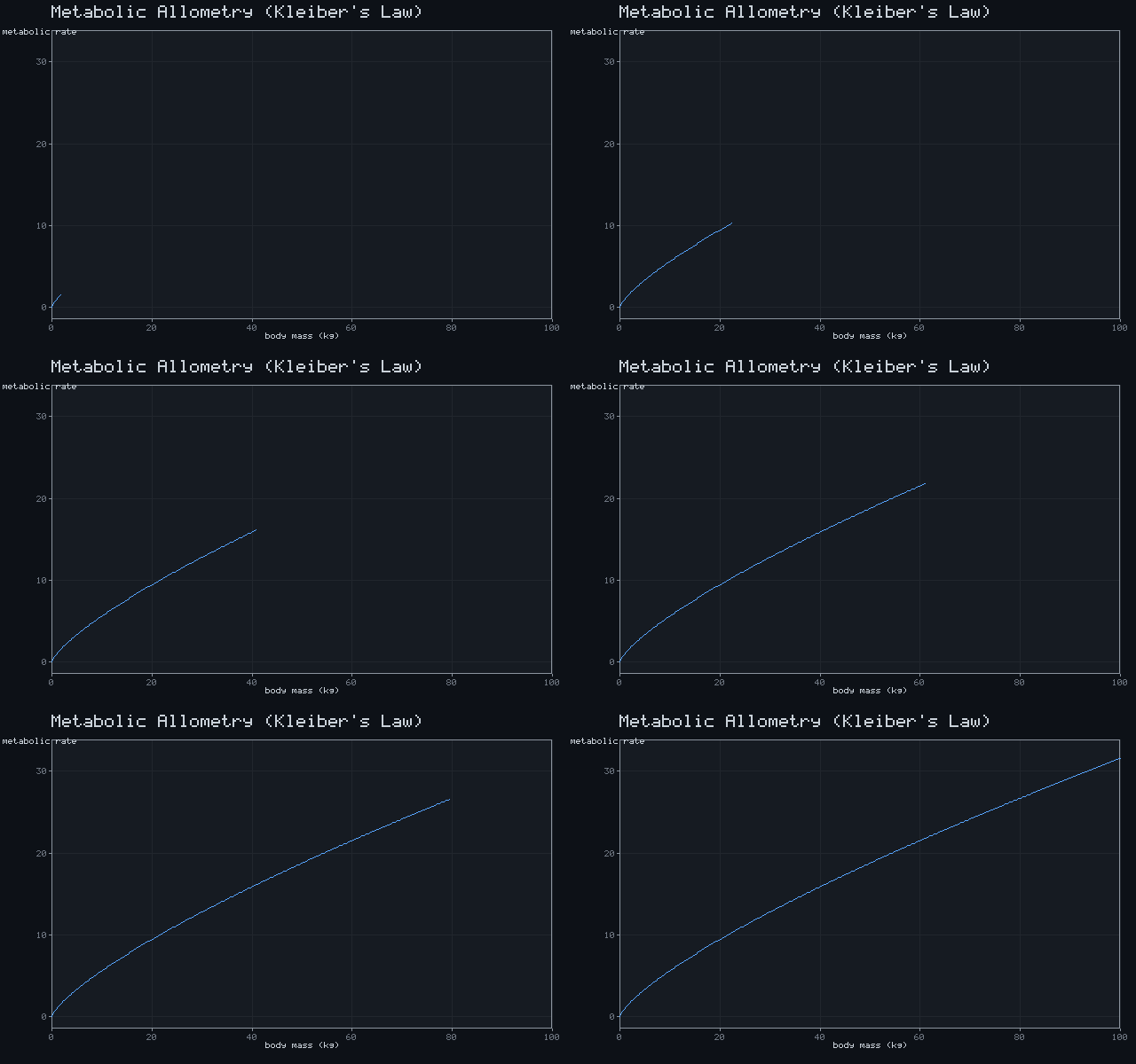

Metabolic Allometry (Kleiber's Law)

BMR ∝ M^¾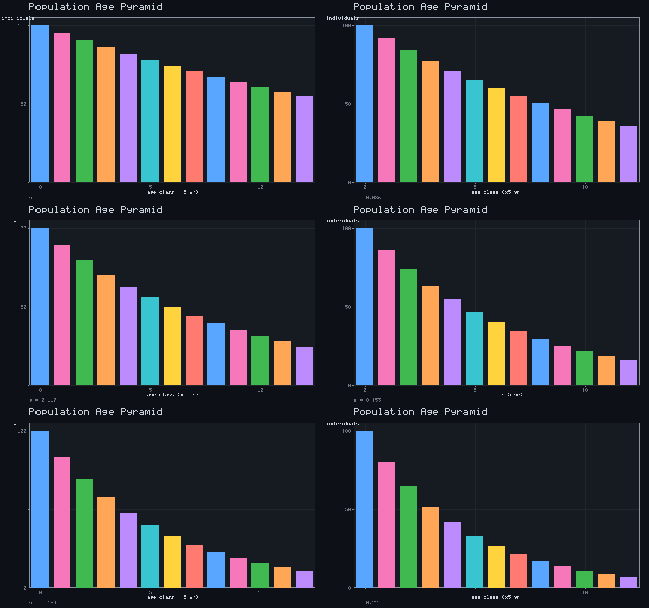

Population Age Pyramid

Nₓ ∝ e^(−g·x)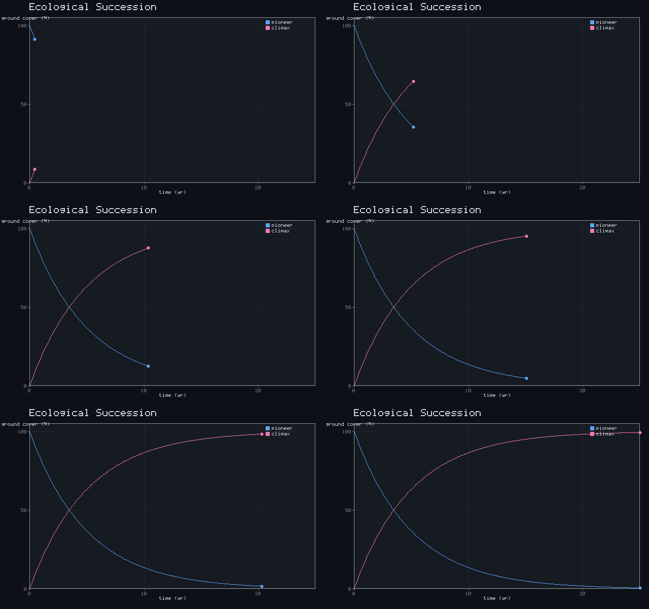

Ecological Succession

pioneer e^(−kt) → climax 1 − e^(−kt)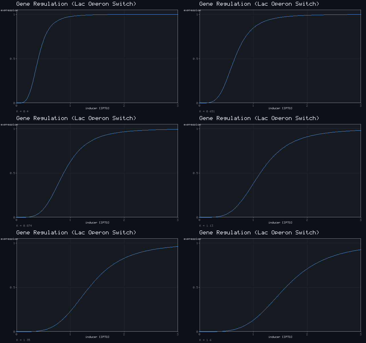

Gene Regulation (Lac Operon Switch)

expression = xⁿ / (xⁿ + Kⁿ), n = 4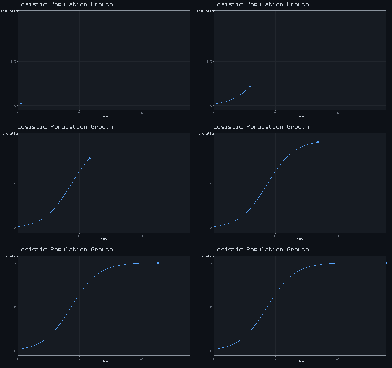

Logistic Population Growth

dN/dt = rN(1 − N/K)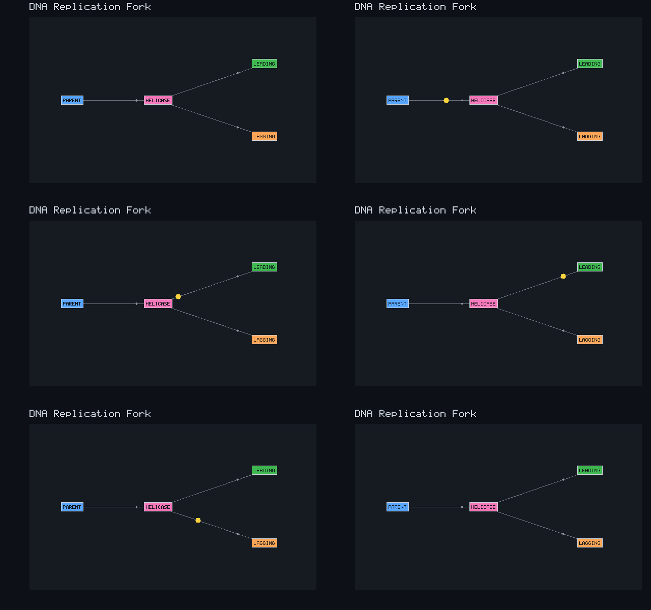

DNA Replication Fork

3'→5' template, leading + lagging

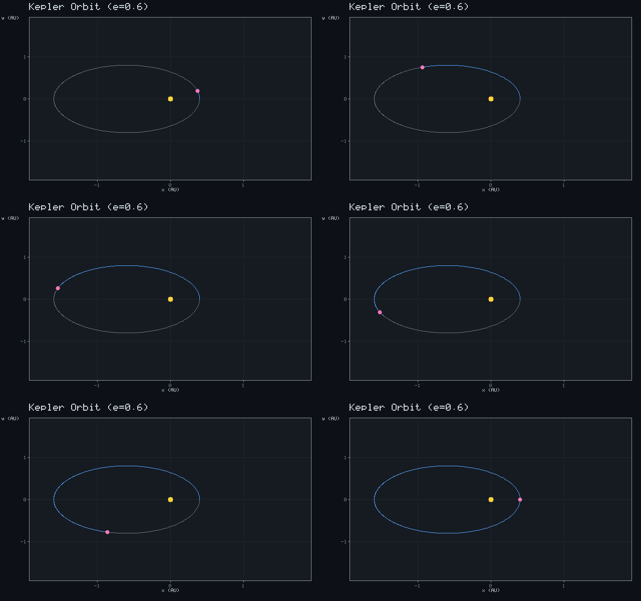
Kepler Orbit (e=0.6)

M = E - e·sin E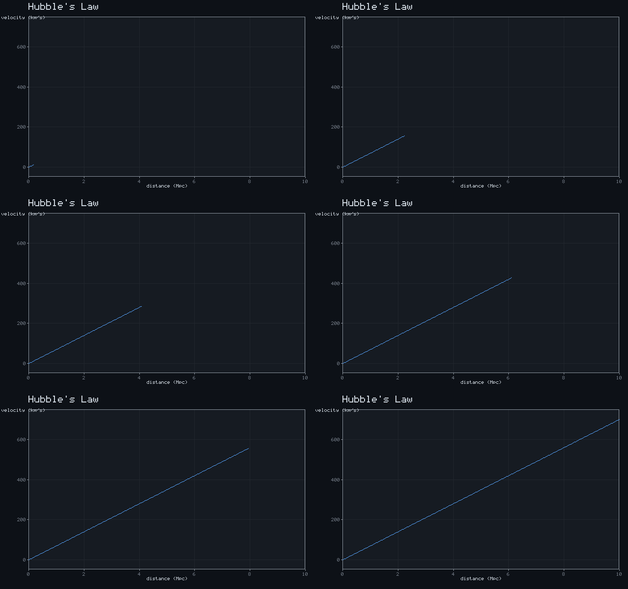

Hubble's Law

v = H₀ d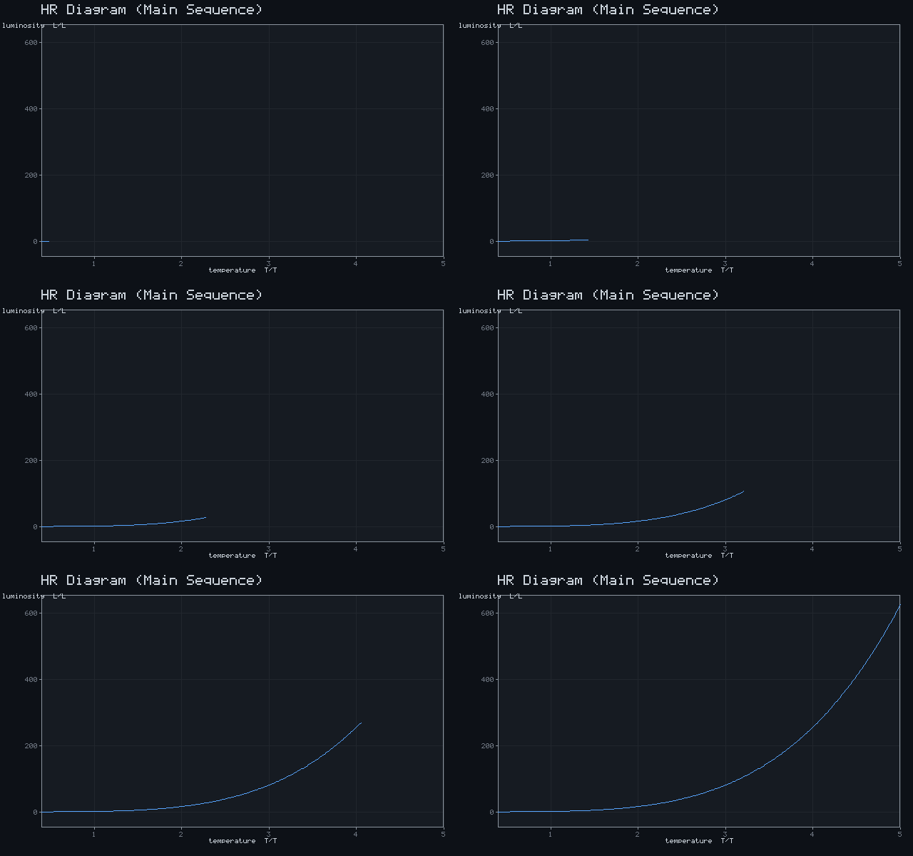

HR Diagram (Main Sequence)

L/L☉ ≈ (T/T☉)⁴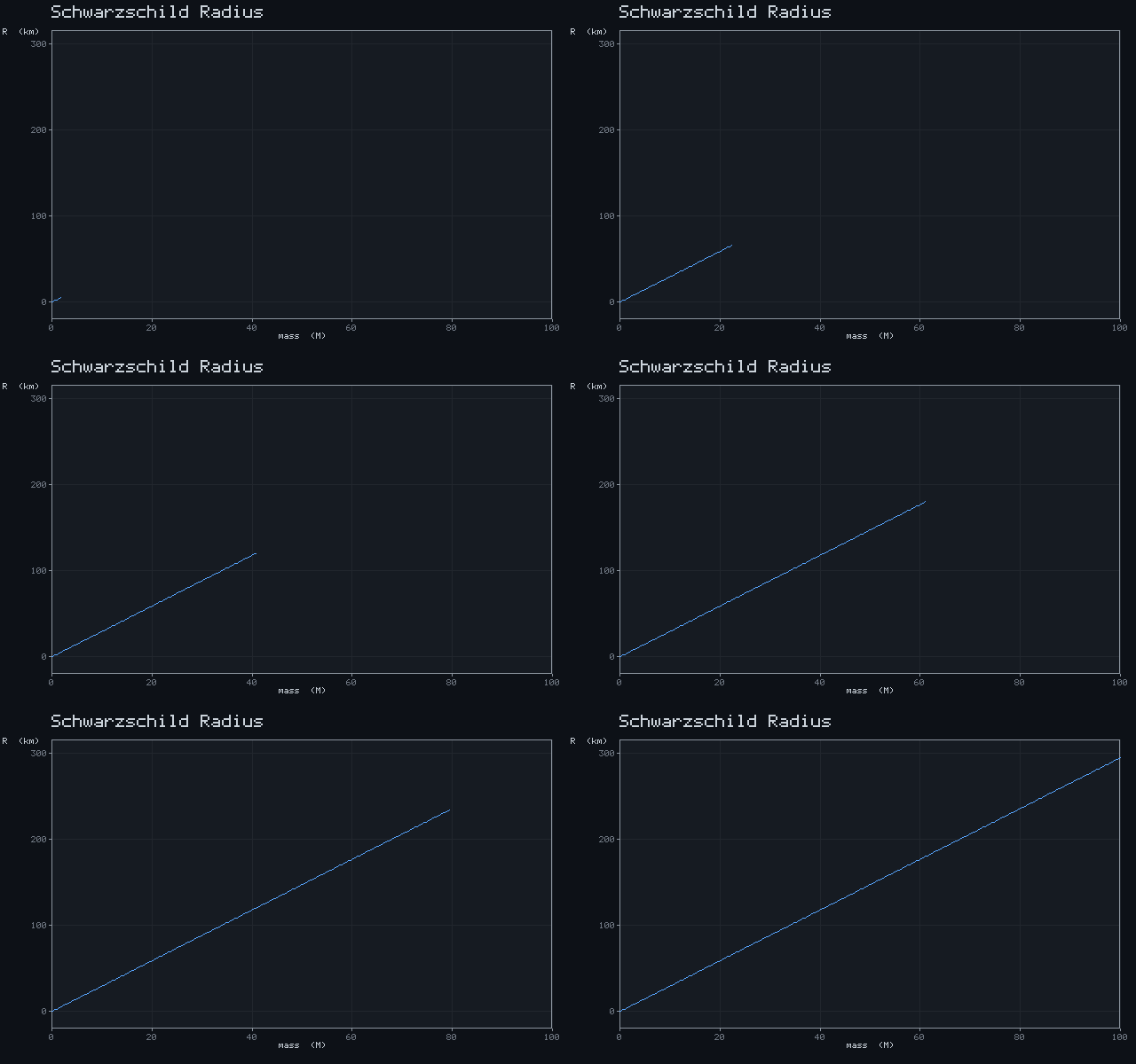

Schwarzschild Radius

Rₛ = 2GM/c²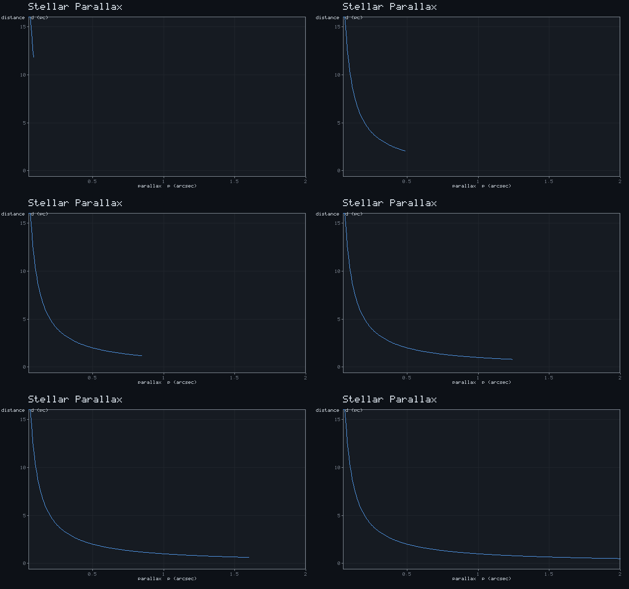

Stellar Parallax

d = 1 / p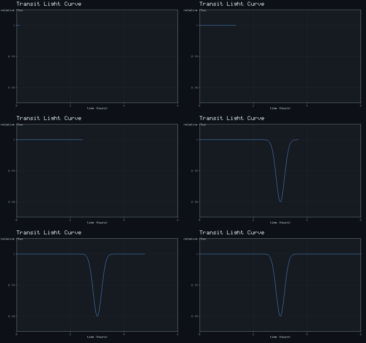

Transit Light Curve

F = 1 − δ·e^(−(t−t₀)²/w)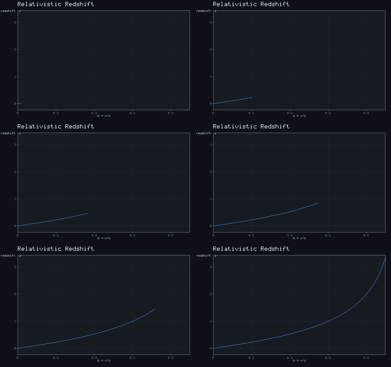

Relativistic Redshift

1 + z = √((1+β)/(1−β)), β = v/c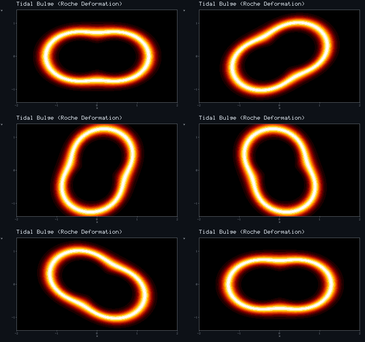

Tidal Bulge (Roche Deformation)

r(θ) = 1 + ε·cos 2(θ − t)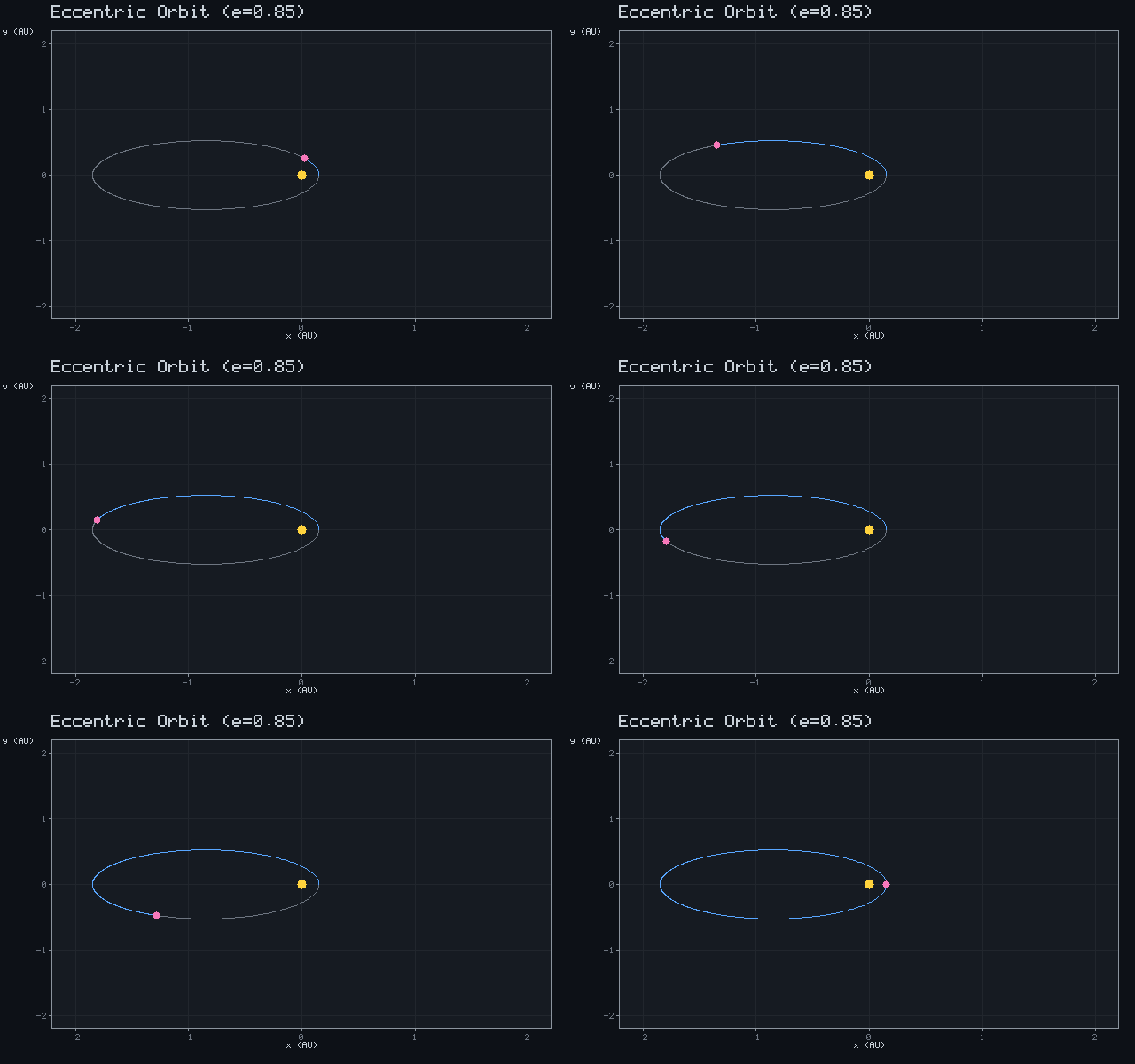

Eccentric Orbit (e=0.85)

M = E − e·sin E, e = 0.85

Normal Distribution

f = 1/(σ√2π) · e^(-x²/2σ²)

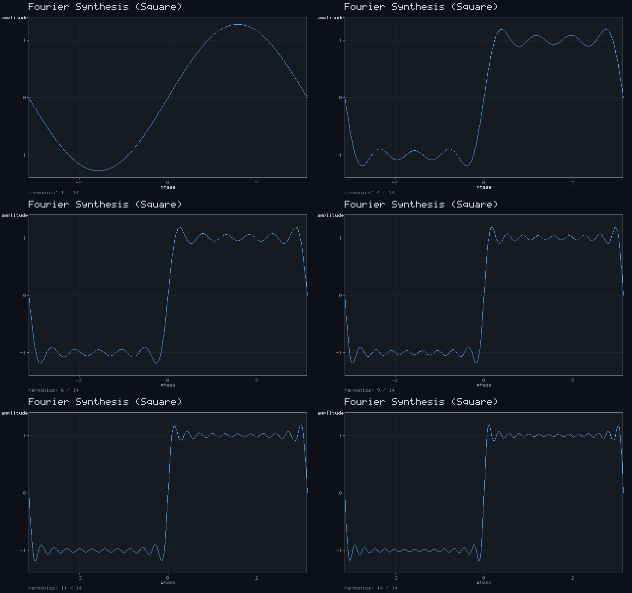
Fourier Synthesis (Square)

f(x) = (4/π) Σ sin((2k-1)x)/(2k-1)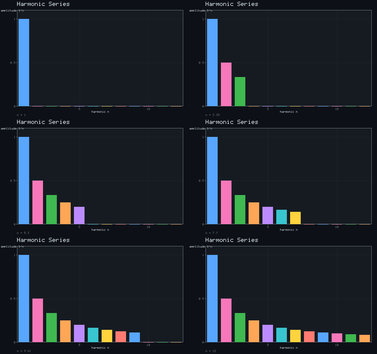

Harmonic Series

Aₙ = 1/n at fₙ = n·f₀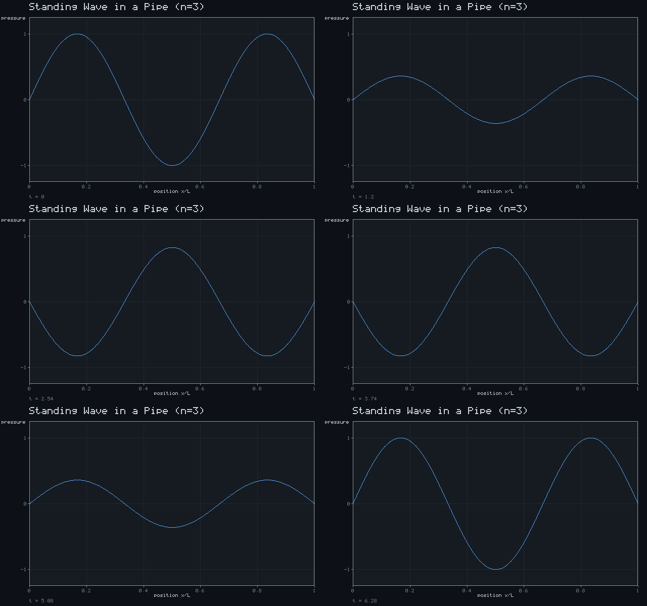

Standing Wave in a Pipe (n=3)

p(x,t) = sin(nπx/L)·cos(ωt), n = 3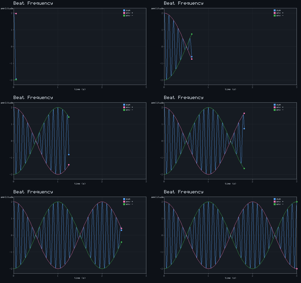

Beat Frequency

cos 2πf₁t + cos 2πf₂t ; f_beat = |f₁−f₂|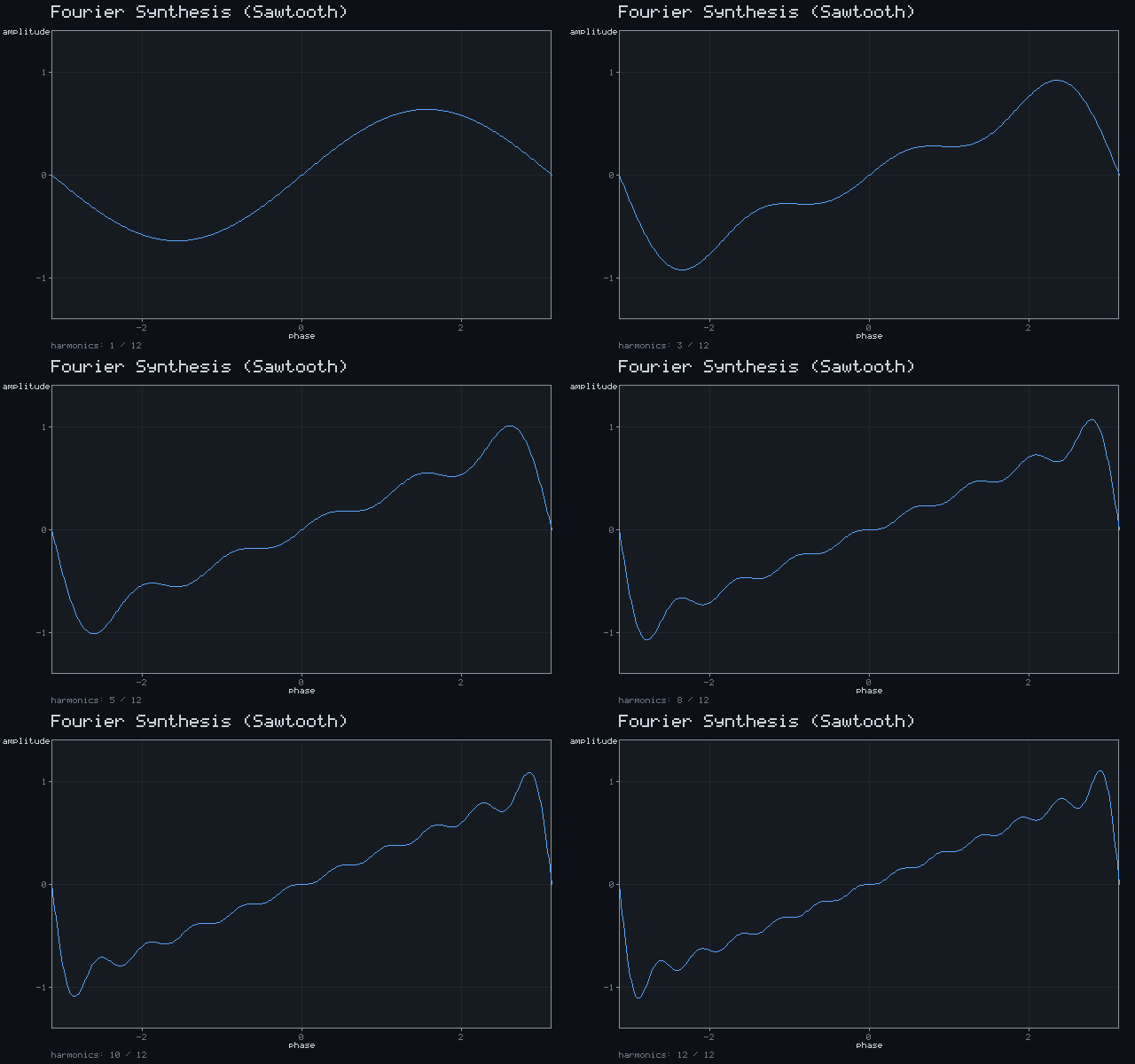

Fourier Synthesis (Sawtooth)

f(x) = (2/π) Σₙ (−1)ⁿ⁺¹ sin(nx)/n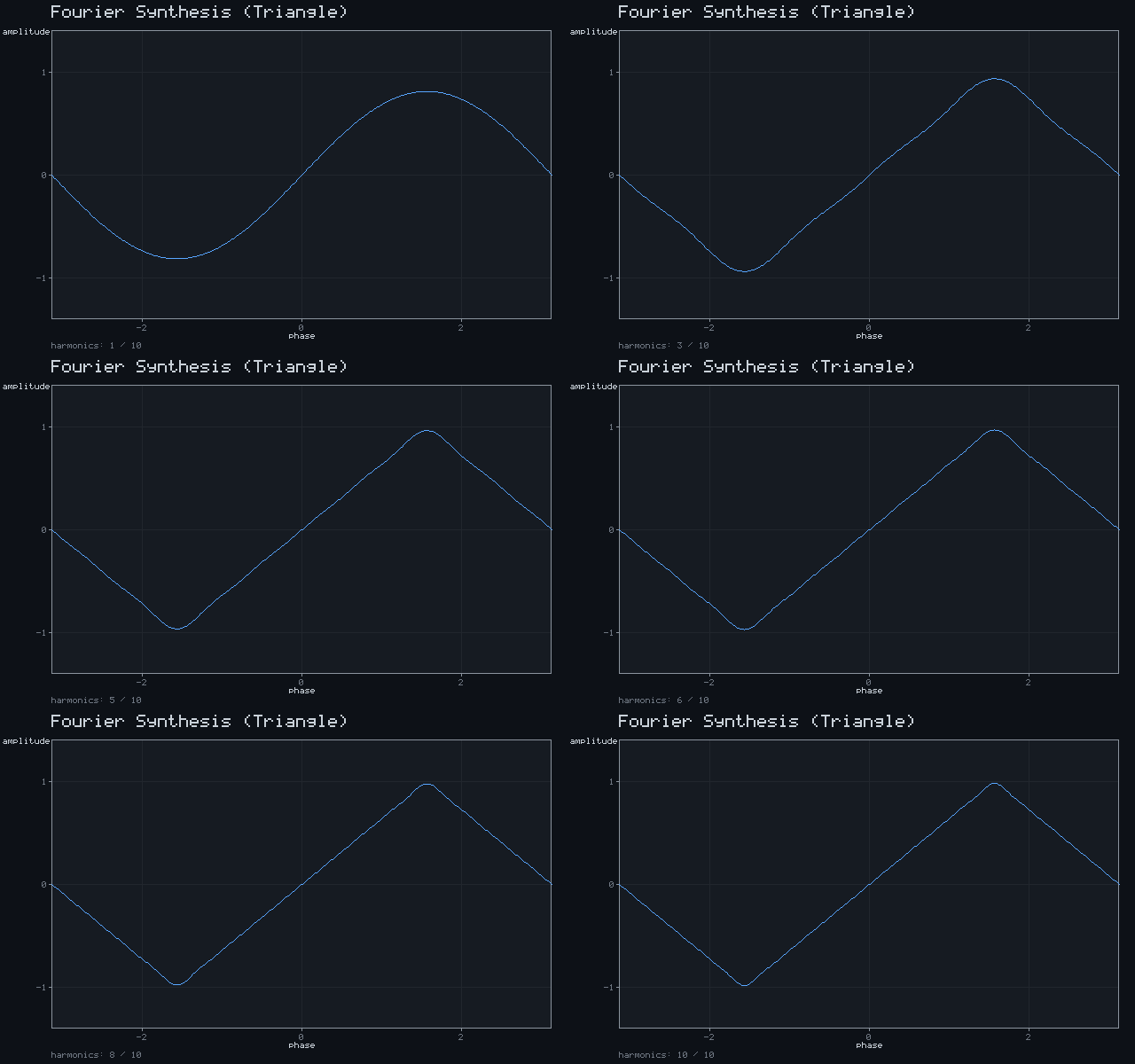

Fourier Synthesis (Triangle)

f(x) = (8/π²) Σ (−1)ᵏ sin((2k+1)x)/(2k+1)²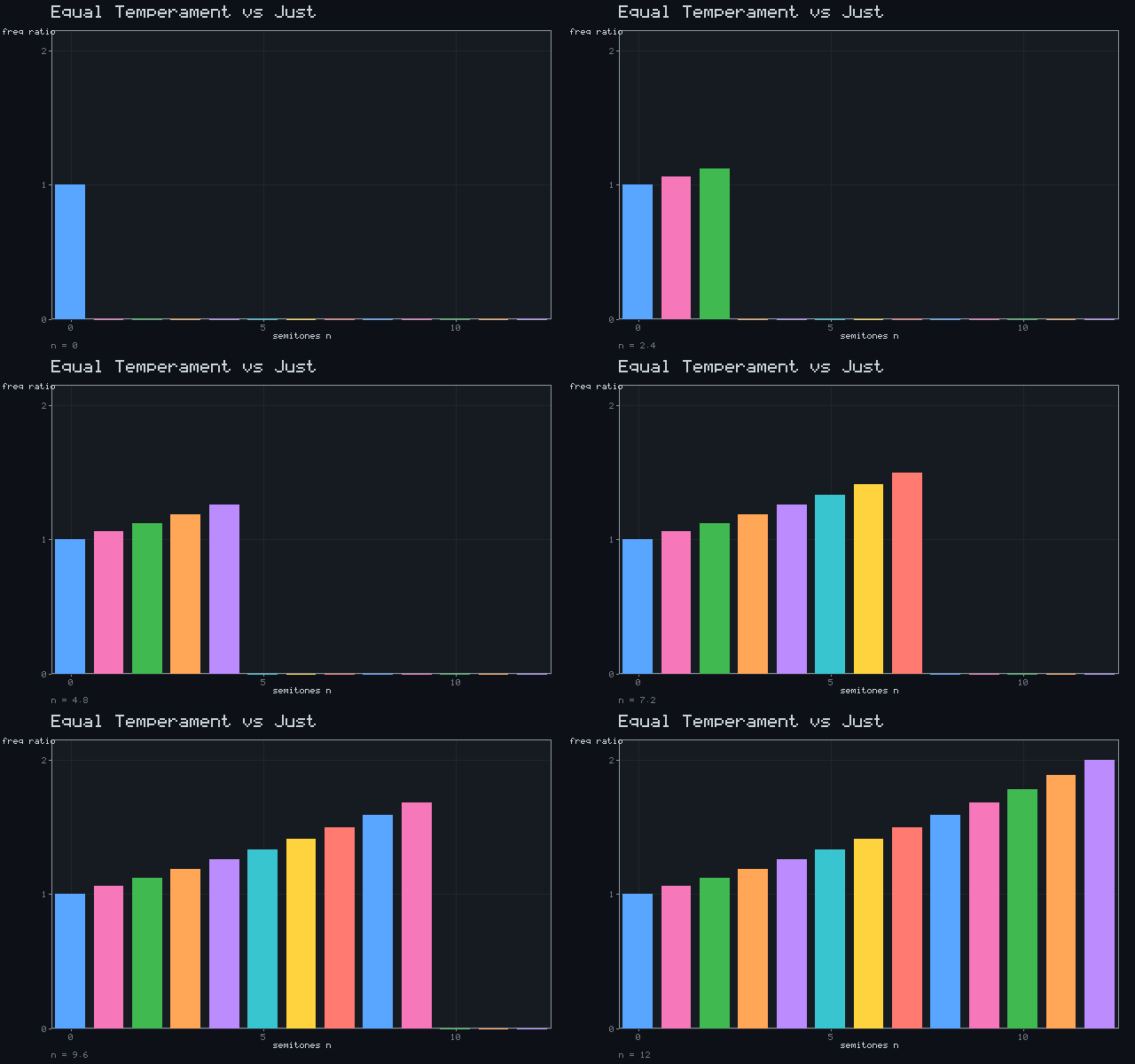

Equal Temperament vs Just

fₙ/f₀ = 2^(n/12)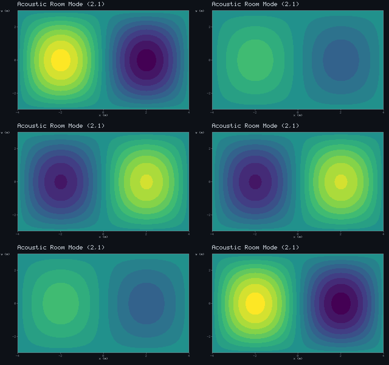

Acoustic Room Mode (2,1)

p = sin(mπx/Lₓ)·sin(nπy/L_y)·cos(ωt)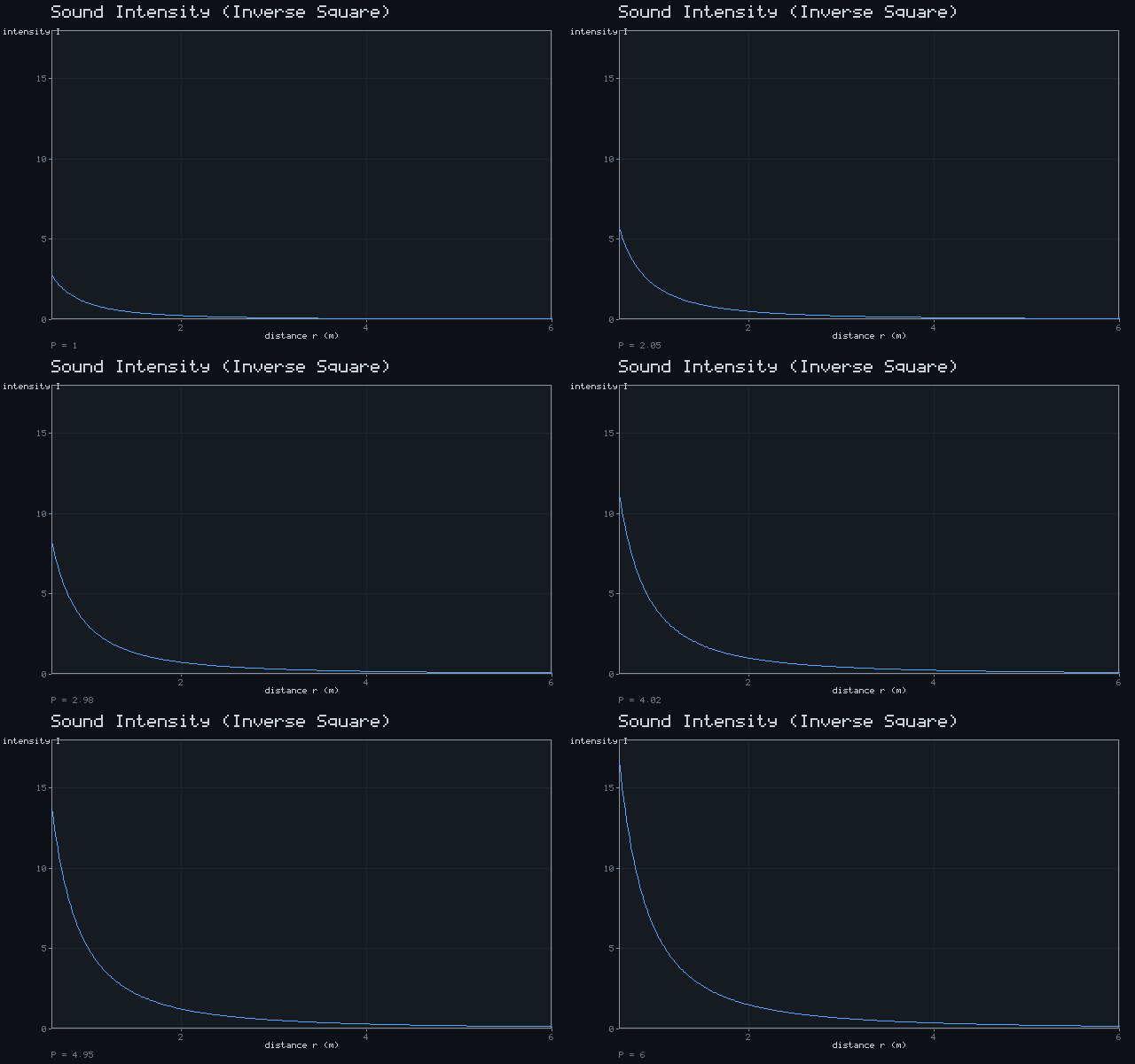

Sound Intensity (Inverse Square)

I = P / (4π r²) ∝ 1/r²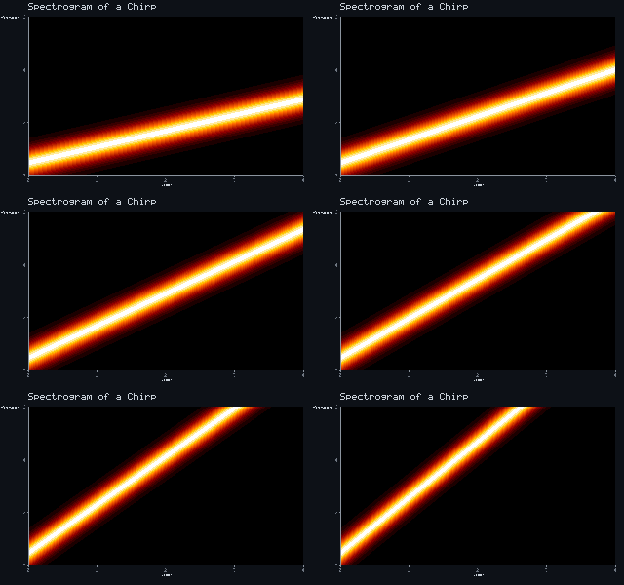

Spectrogram of a Chirp

frequency rising with time

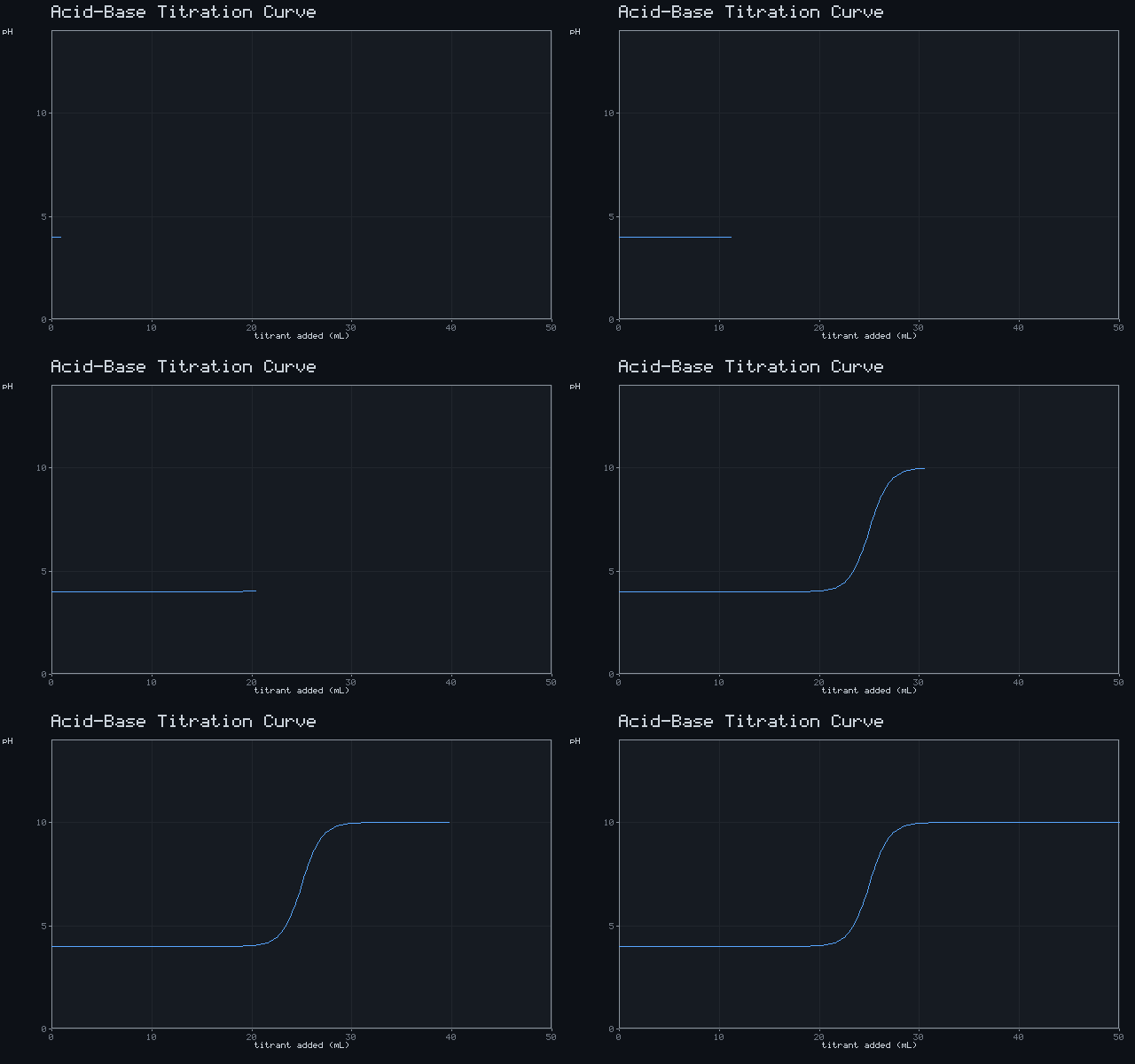
Acid-Base Titration Curve

pH = 7 + 3·tanh((V − Vₑ)/2)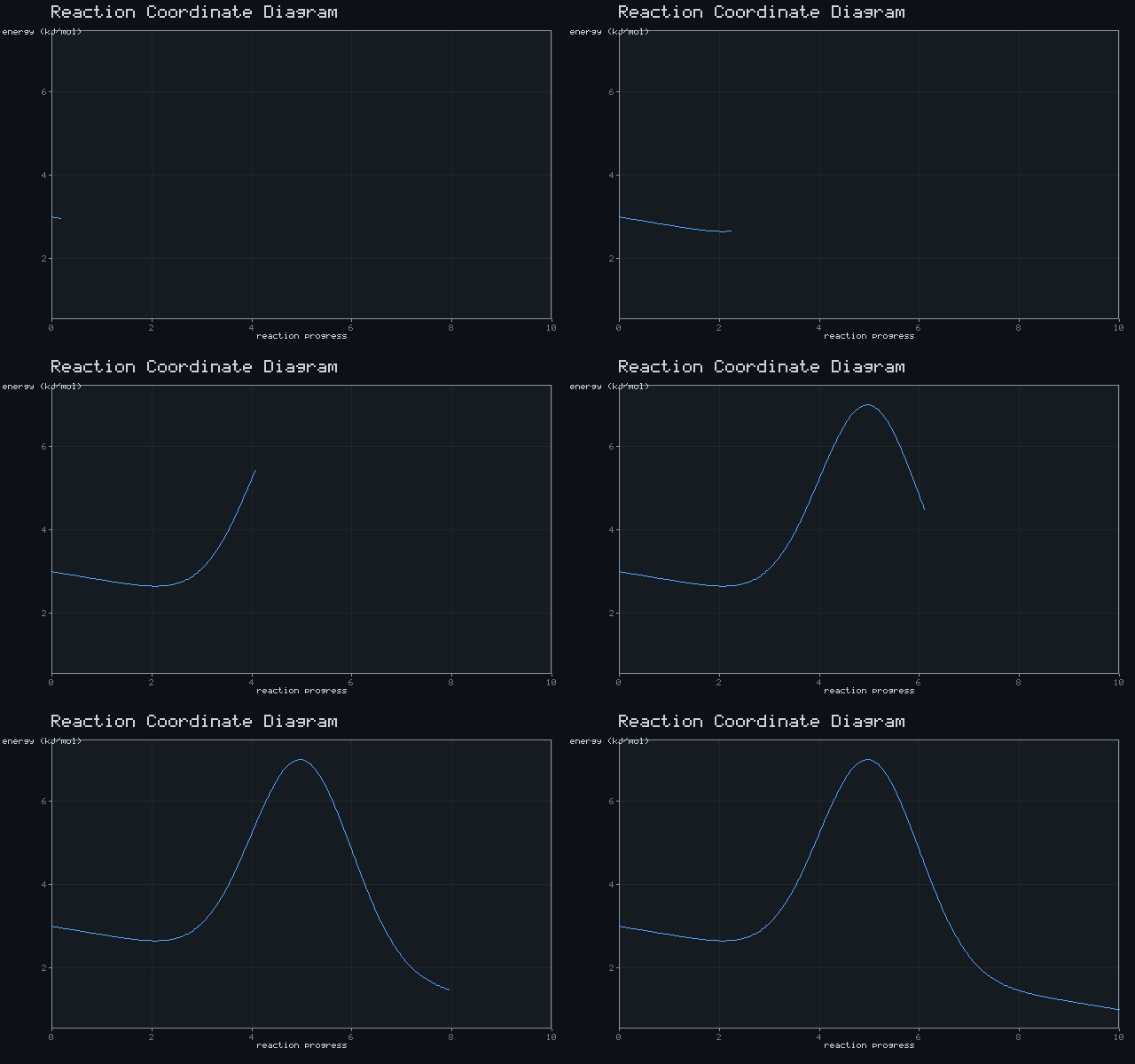

Reaction Coordinate Diagram

E(ξ) = ΔE·ξ + Eₐ·exp(−(ξ−ξ‡)²/2σ²)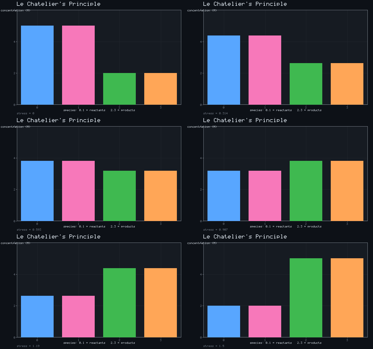

Le Chatelier's Principle

A + B ⇌ C + D (stress → shift toward products)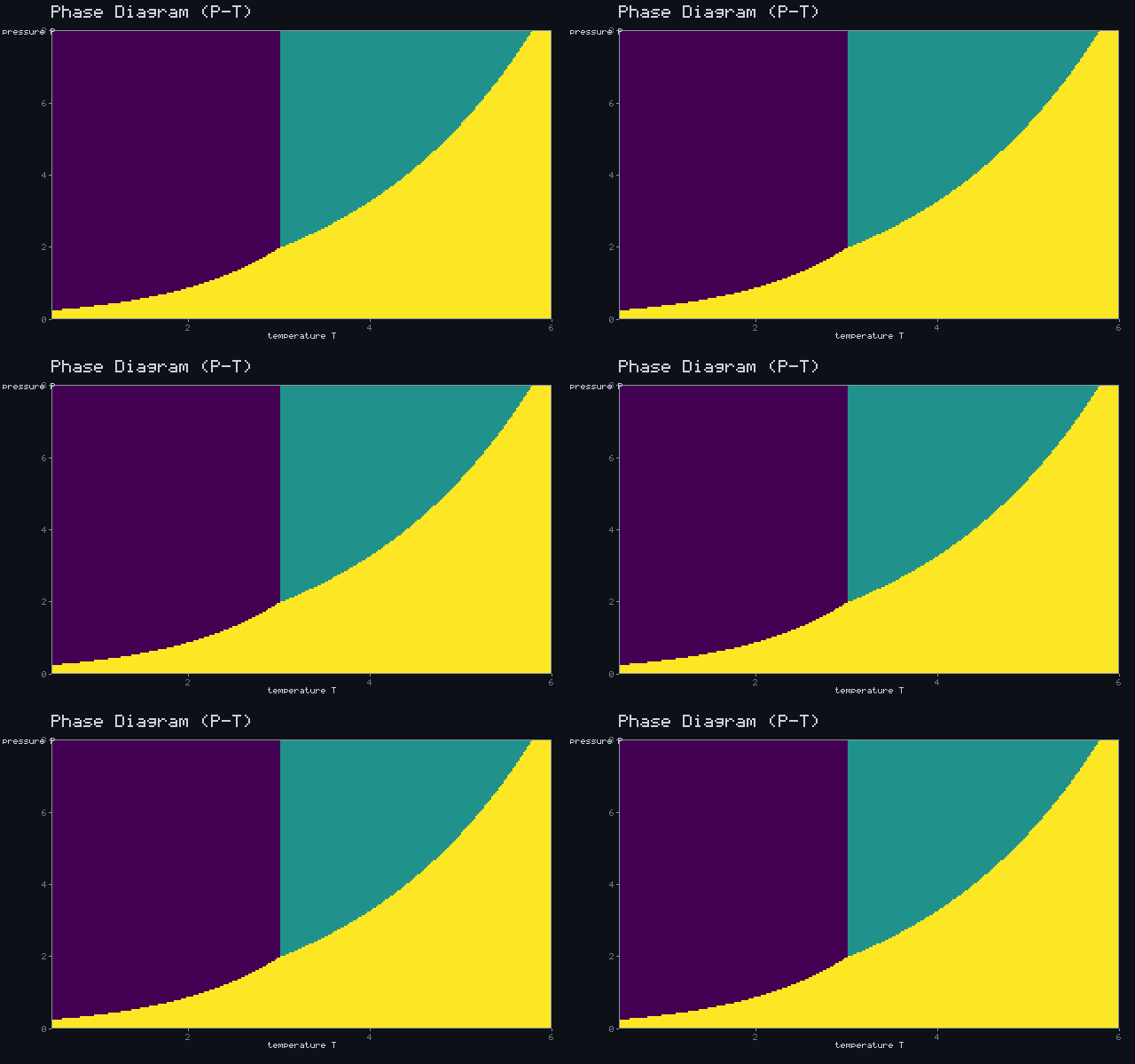

Phase Diagram (P-T)

regions bounded by the sublimation, melting & vaporization curves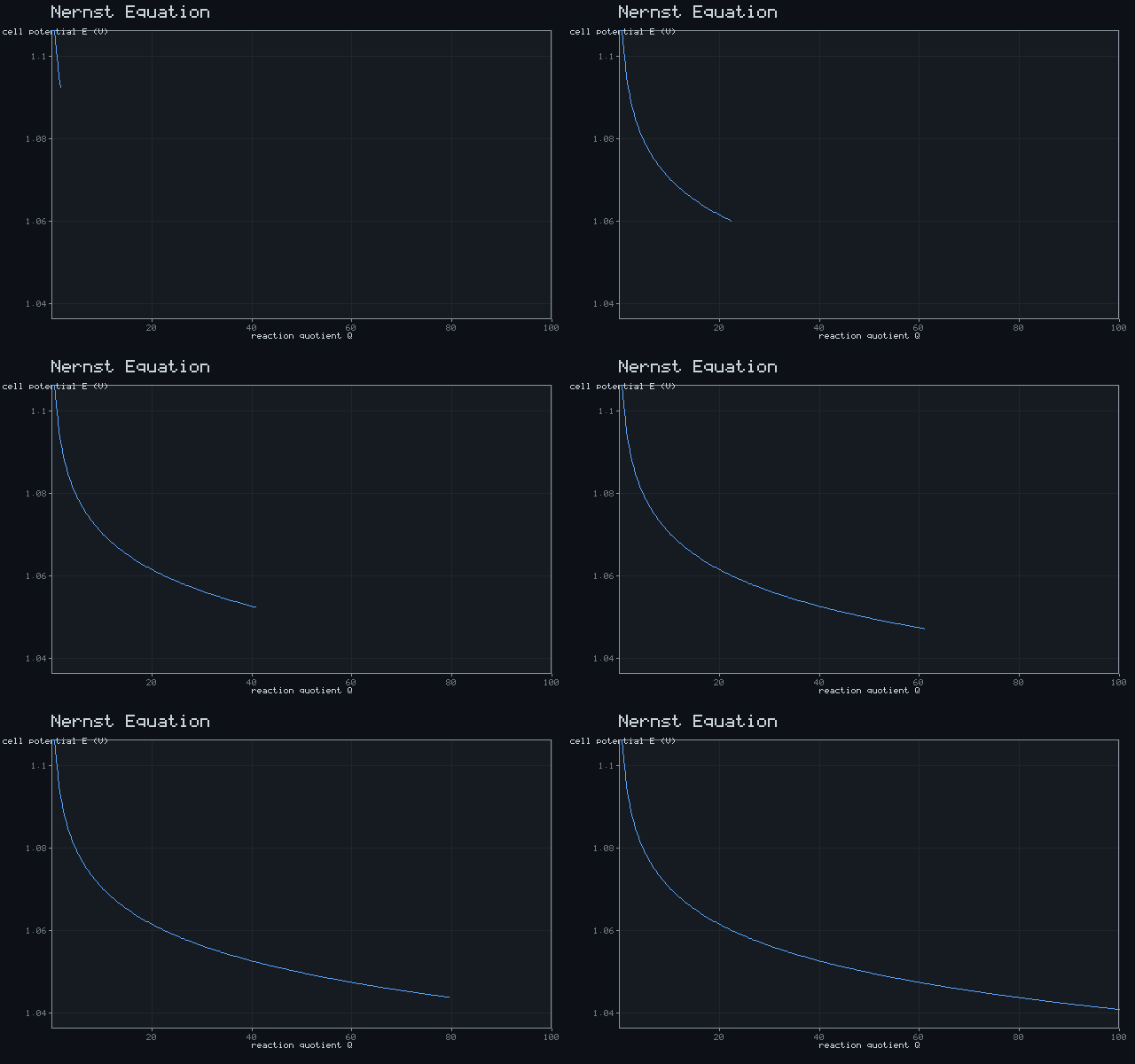

Nernst Equation

E = E° − (RT/nF)·ln Q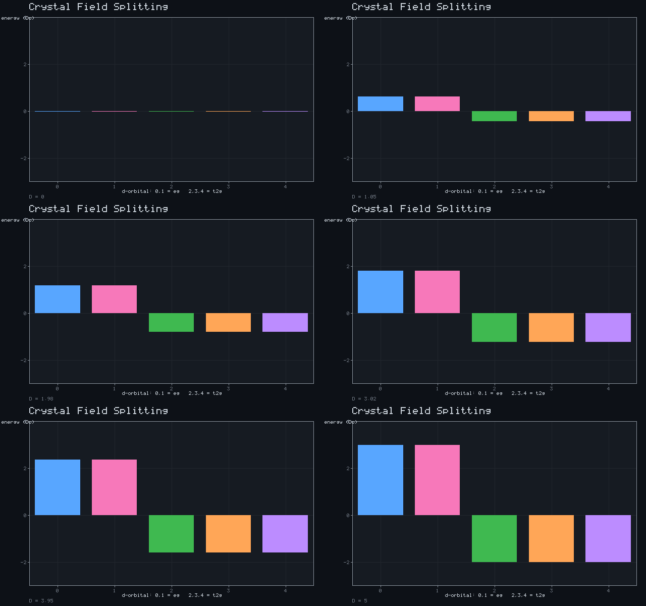

Crystal Field Splitting

e_g: +0.6·Δₒ · t₂g: −0.4·Δₒ (octahedral)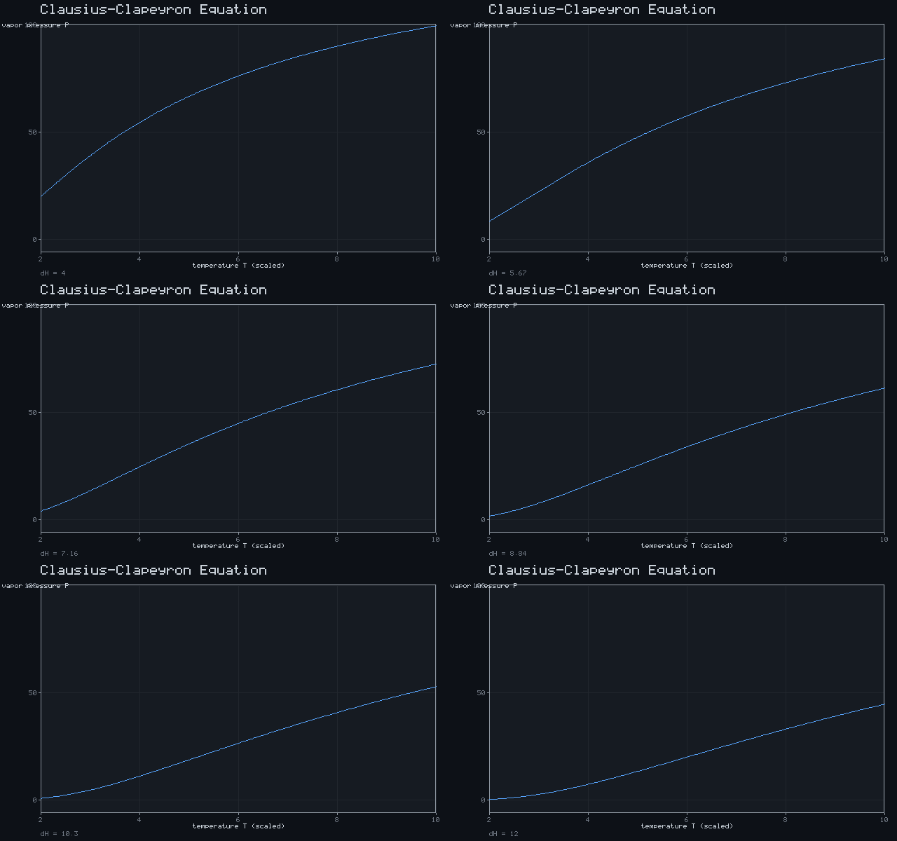

Clausius-Clapeyron Equation

ln P = A − ΔH_vap /(R·T)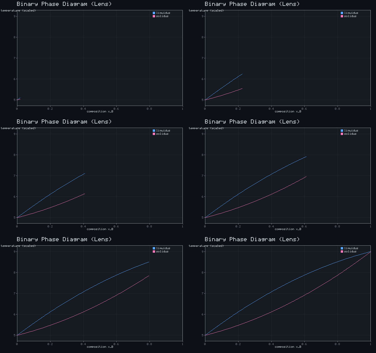

Binary Phase Diagram (Lens)

liquidus & solidus vs. composition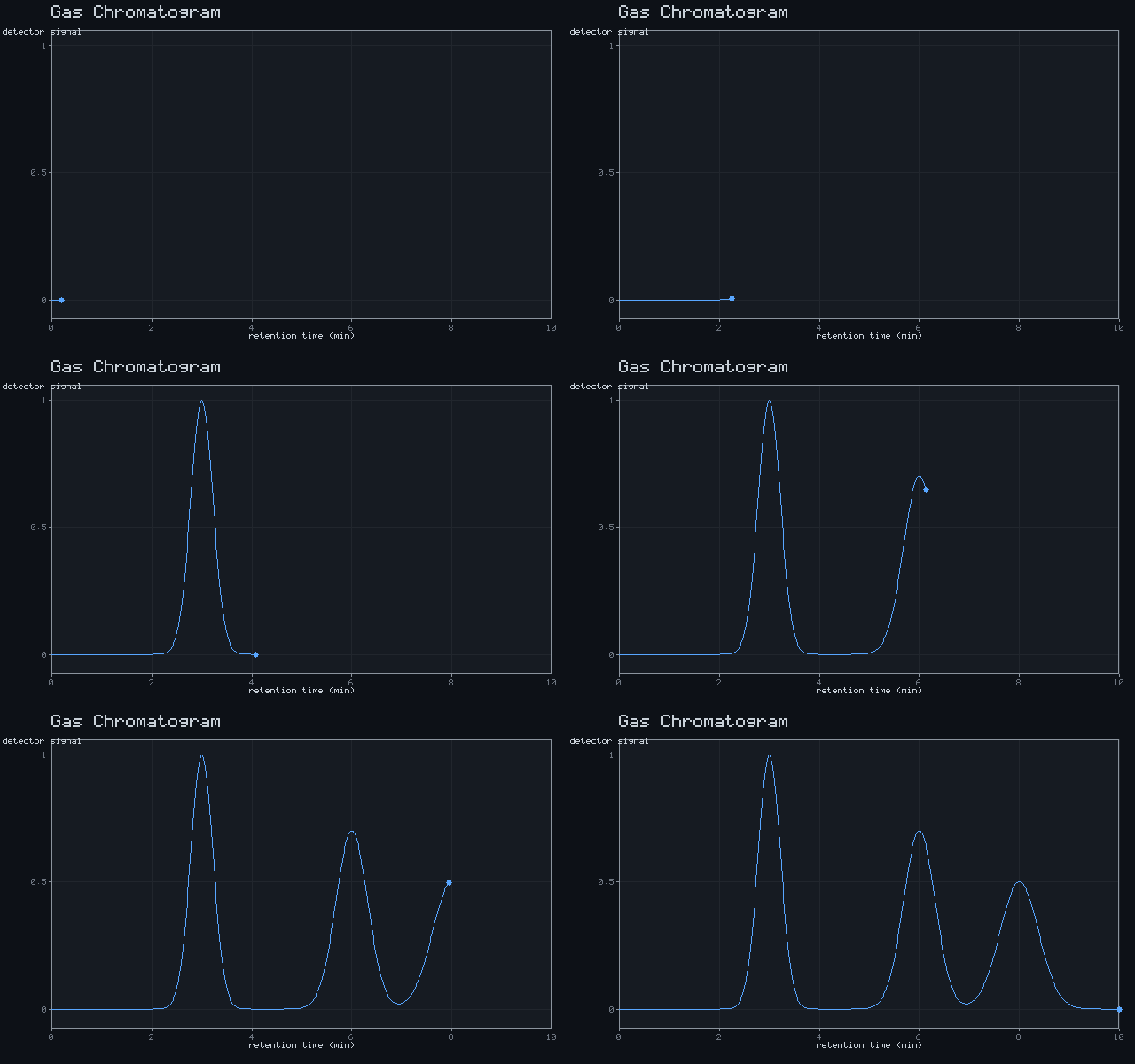

Gas Chromatogram

signal = Σ Aᵢ·exp(−(t − t_R,i)²/2σ²)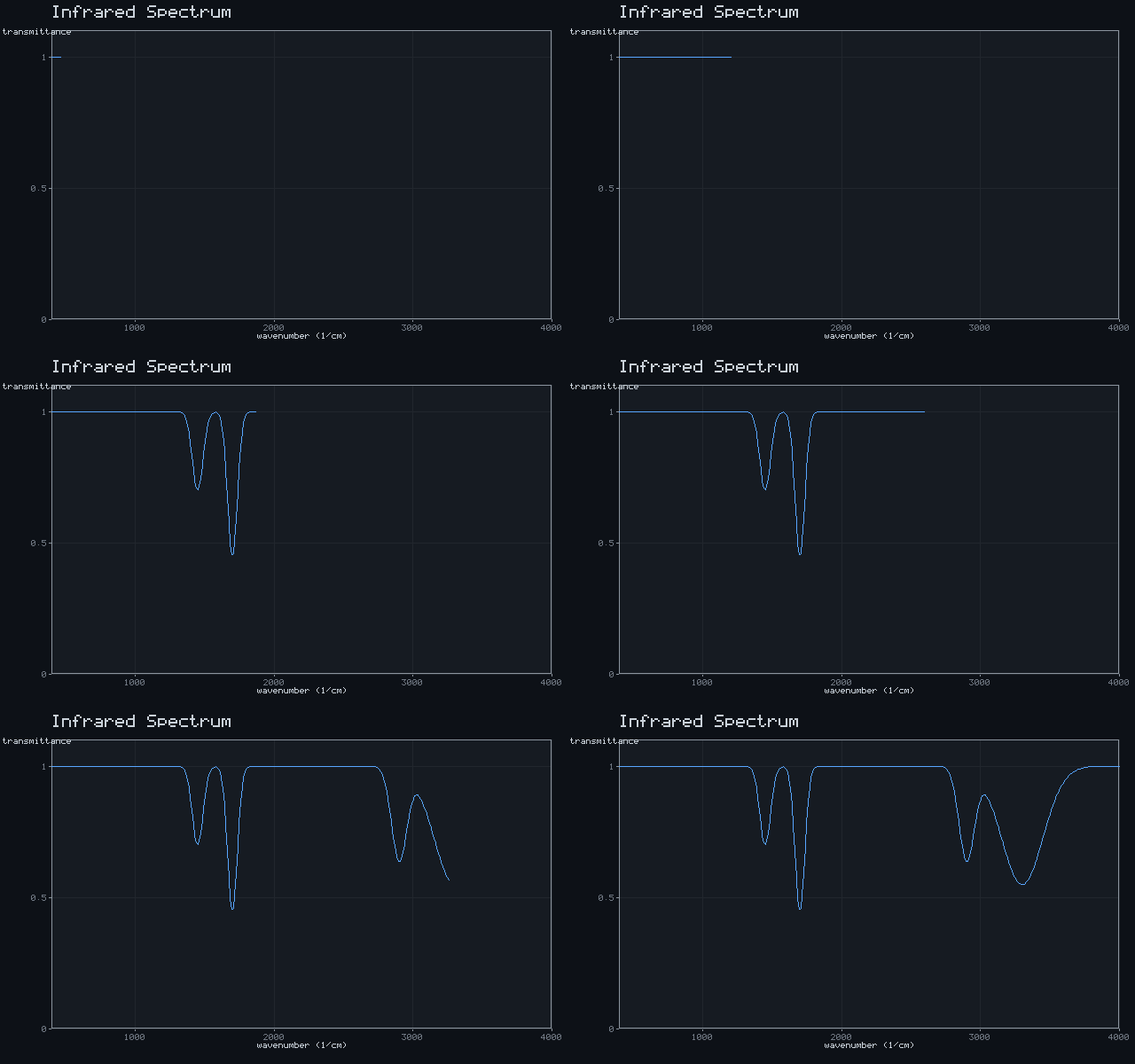

Infrared Spectrum

T(ν̃) = 1 − Σ Aᵢ·exp(−(ν̃ − ν̃ᵢ)²/2σᵢ²)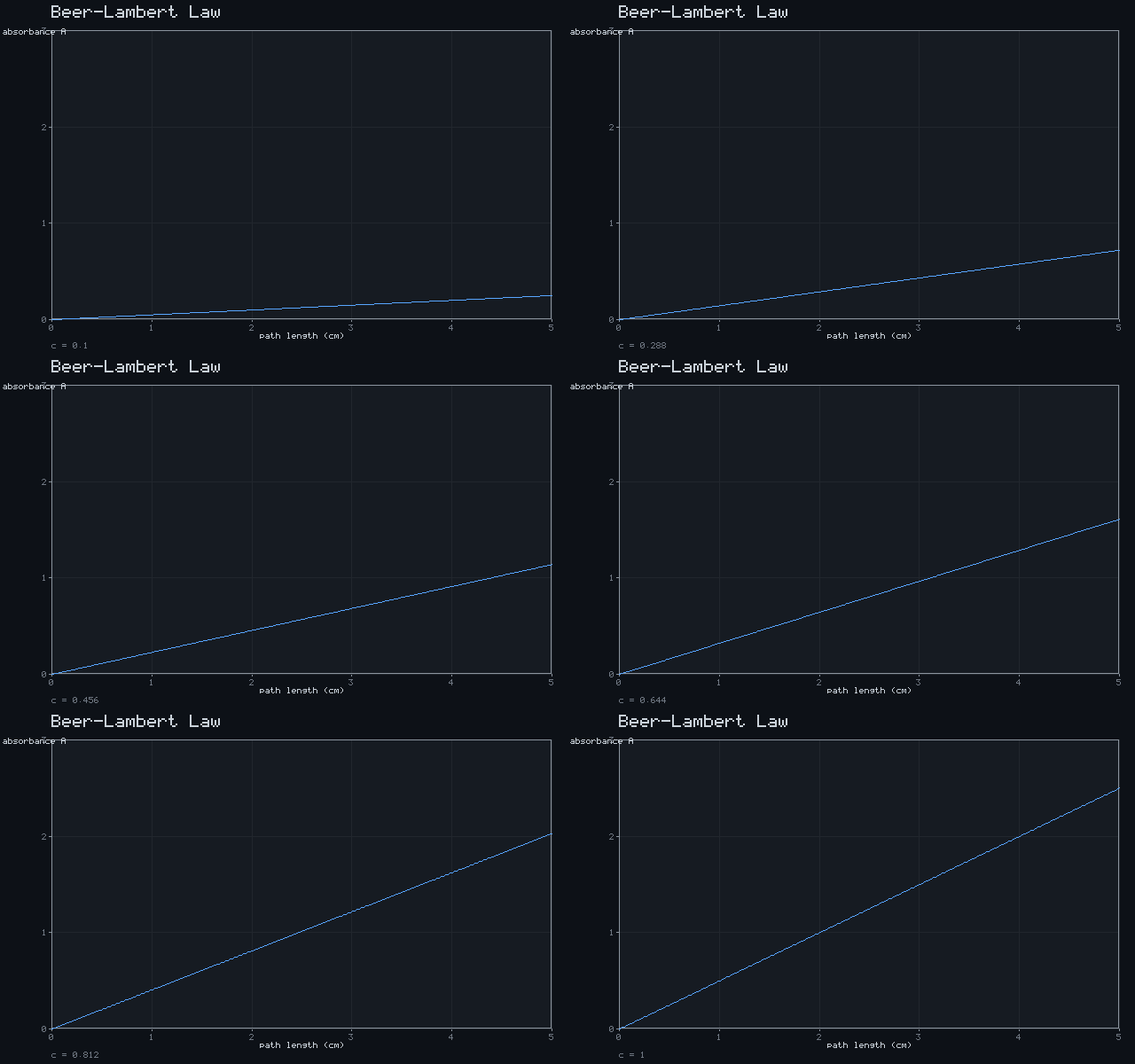

Beer-Lambert Law

A = ε·c·ℓ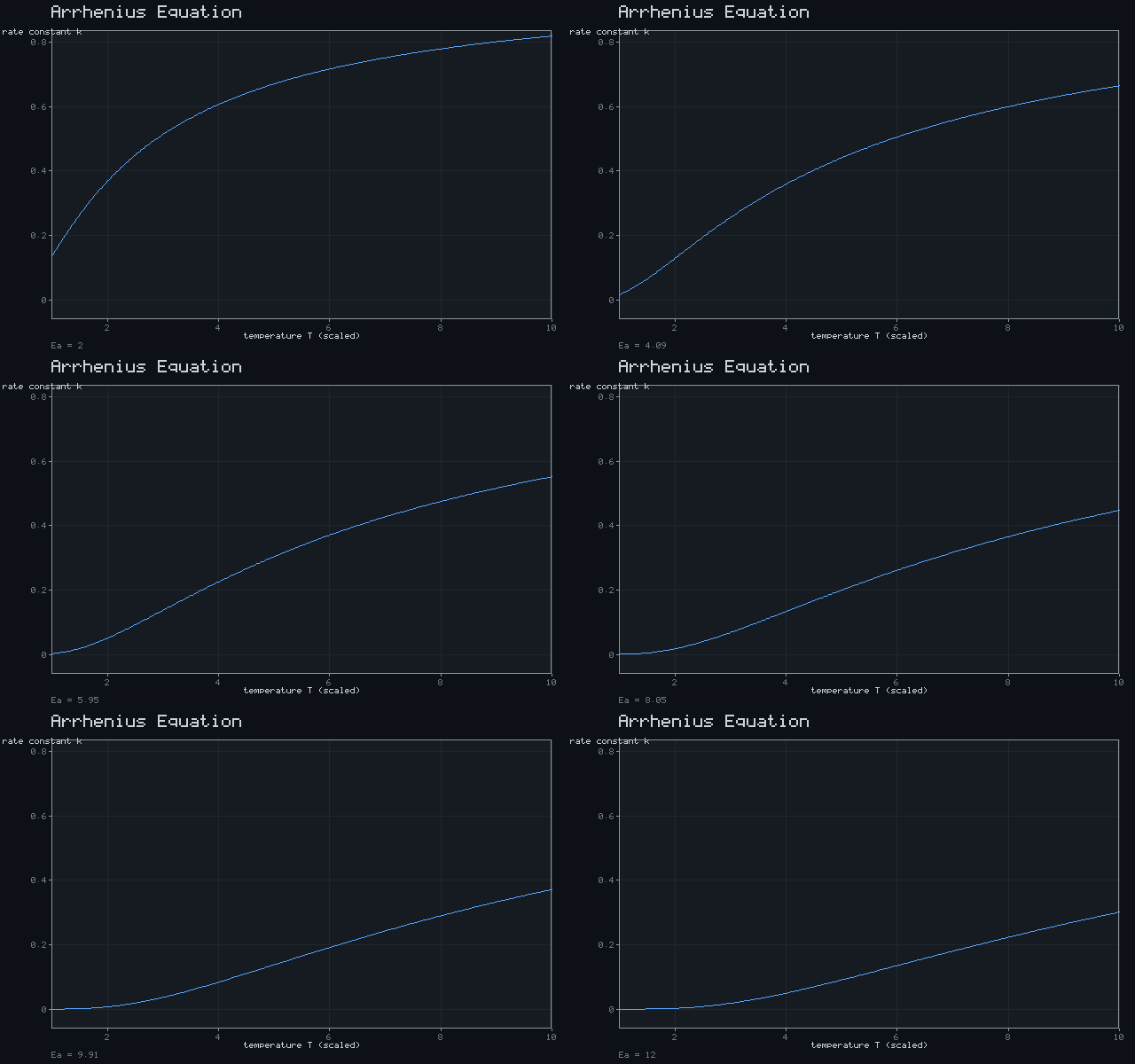

Arrhenius Equation

k = A·exp(−Eₐ /(R·T))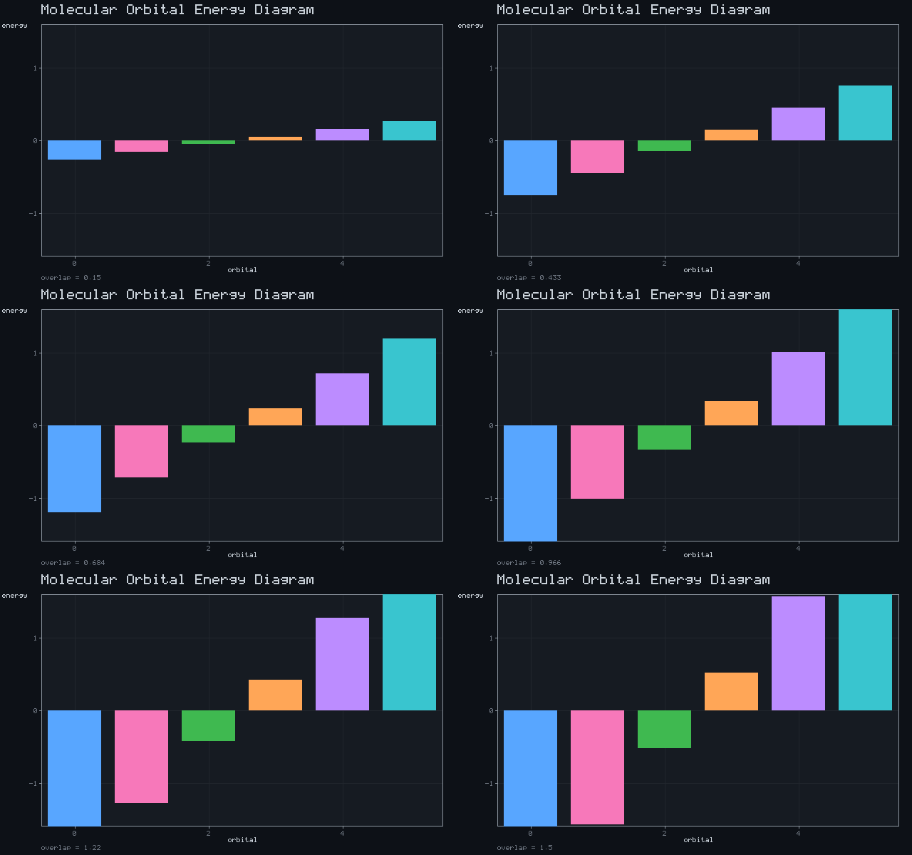

Molecular Orbital Energy Diagram

σ / σ* splitting vs overlap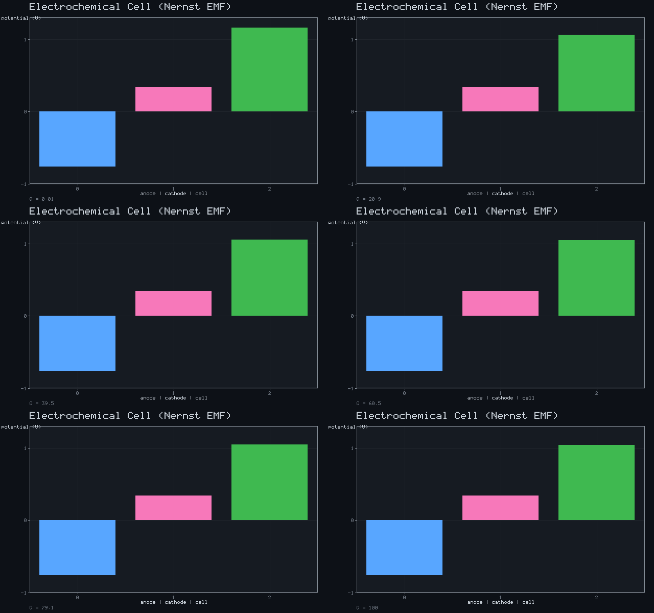

Electrochemical Cell (Nernst EMF)

E_cell = E° − (RT/nF) ln Q

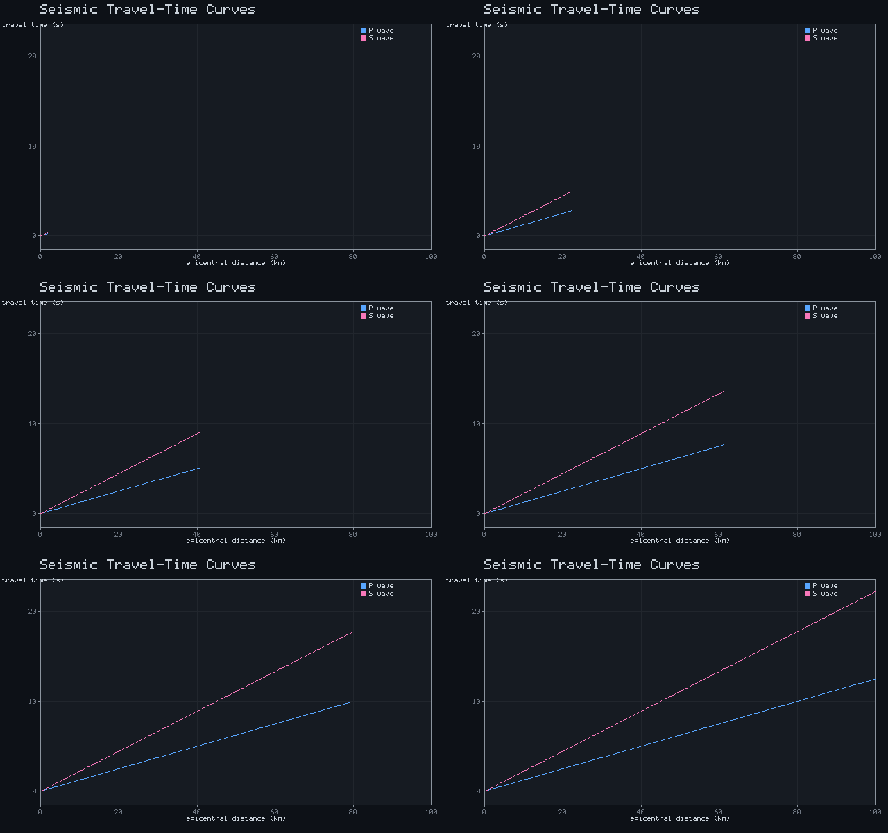
Seismic Travel-Time Curves

t_P = Δ/v_P, t_S = Δ/v_S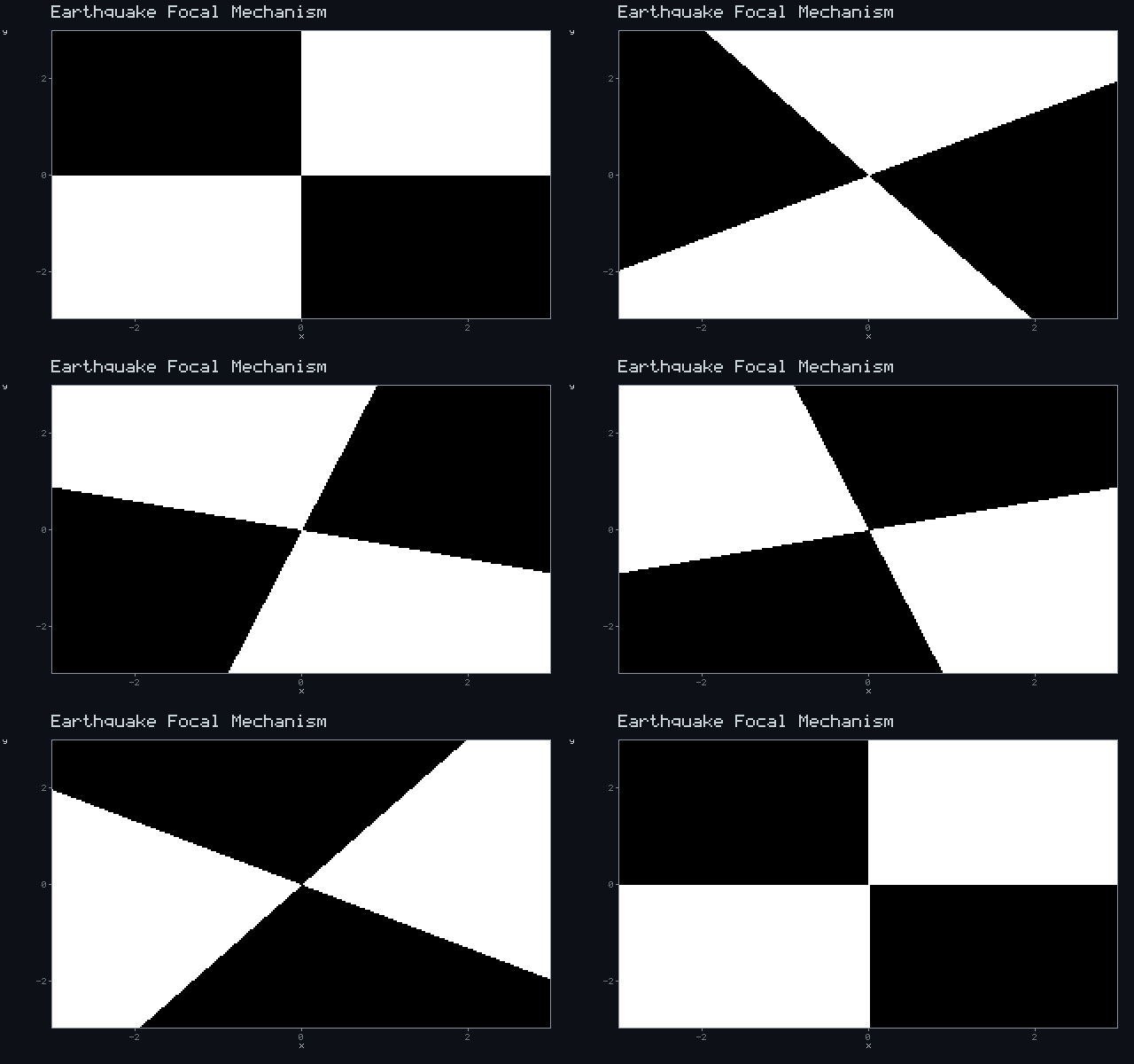

Earthquake Focal Mechanism

sign(sin 2θ) double-couple radiation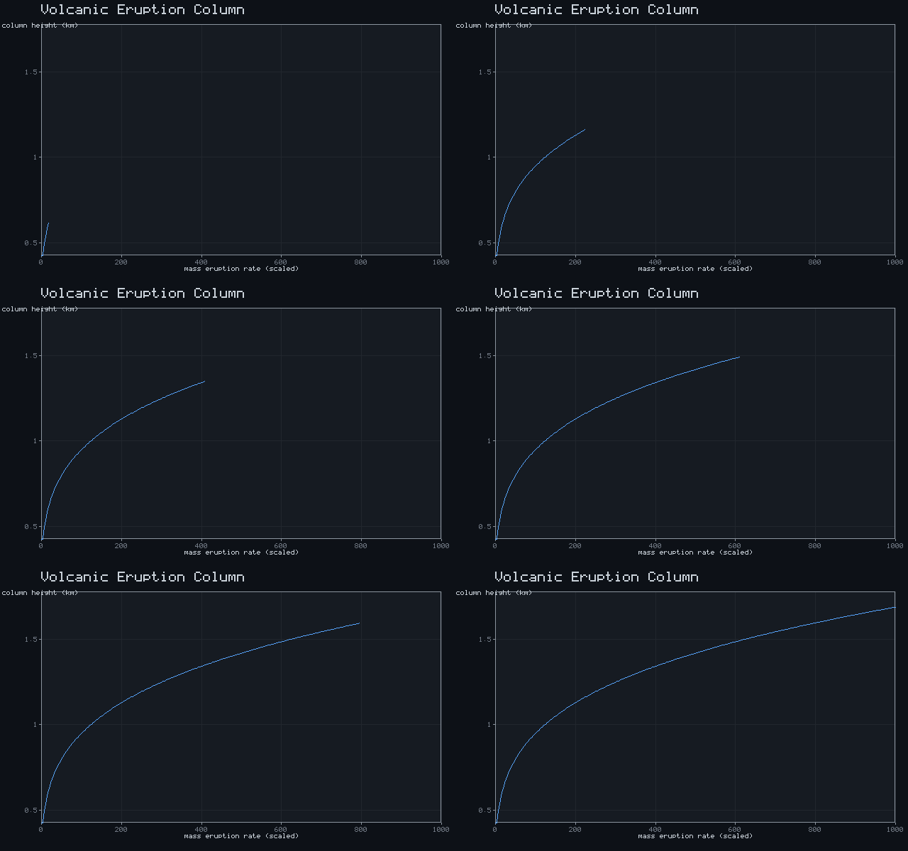

Volcanic Eruption Column

H ≈ 0.3·Q^¼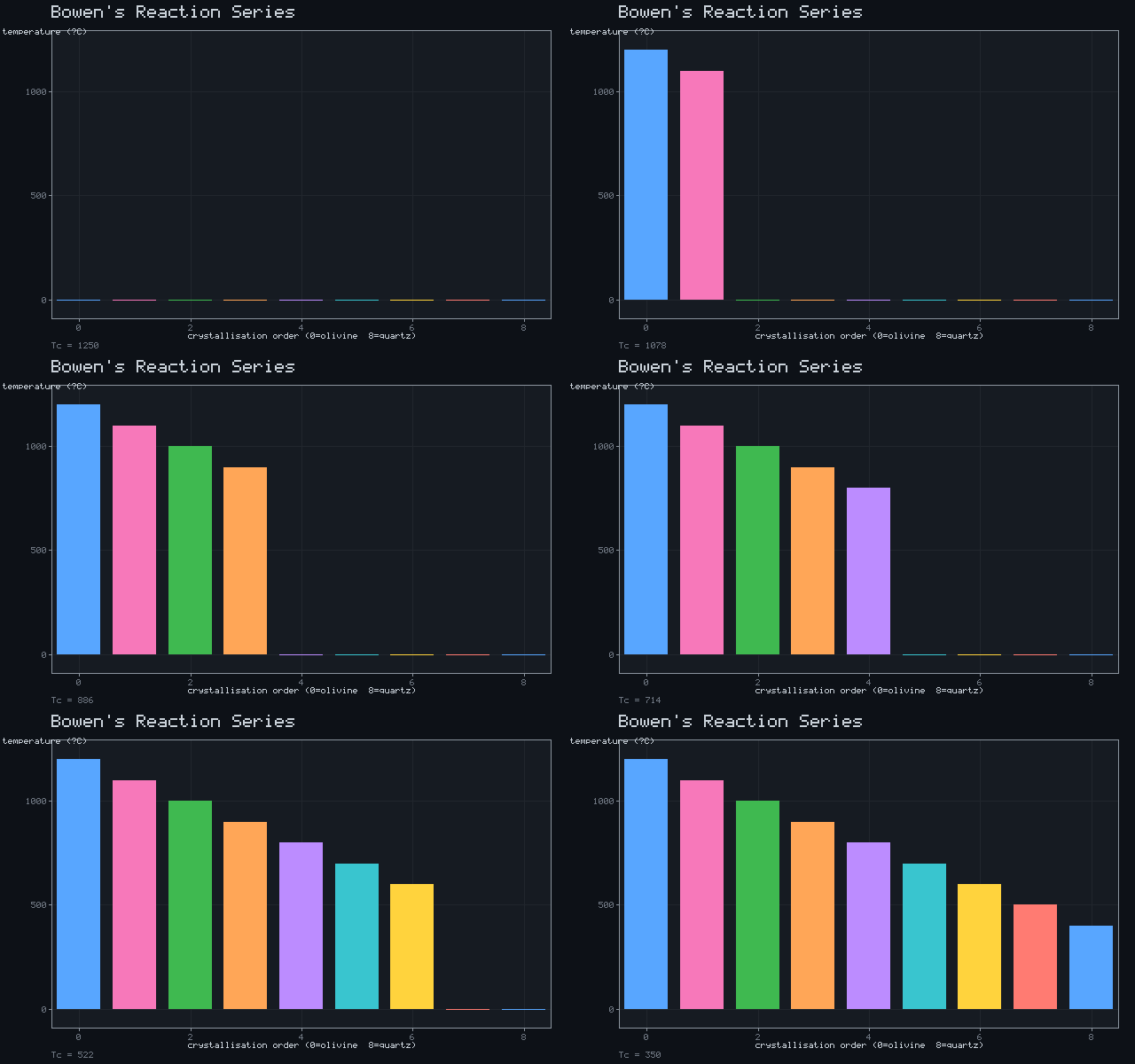

Bowen's Reaction Series

T_crys: olivine → … → quartz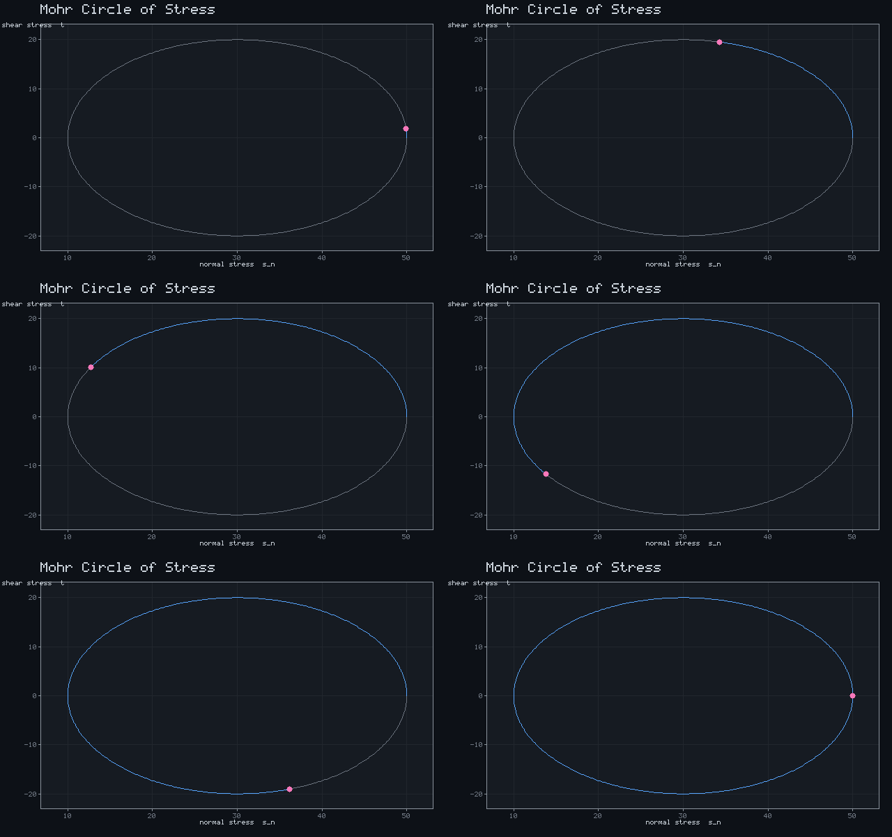

Mohr Circle of Stress

(σ_n − c)² + τ² = R²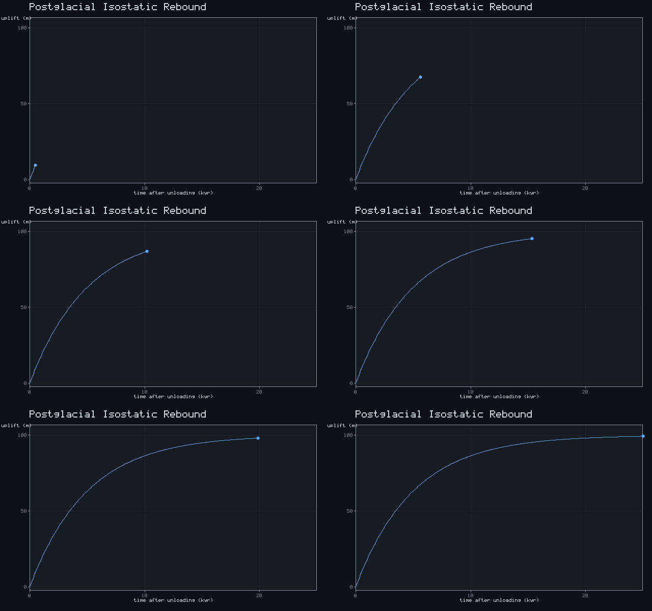

Postglacial Isostatic Rebound

u(t) = u_max·(1 − e^(−t/τ))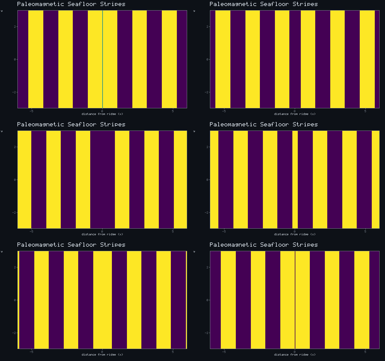

Paleomagnetic Seafloor Stripes

M(x) = sign(sin 3|x|) reversal record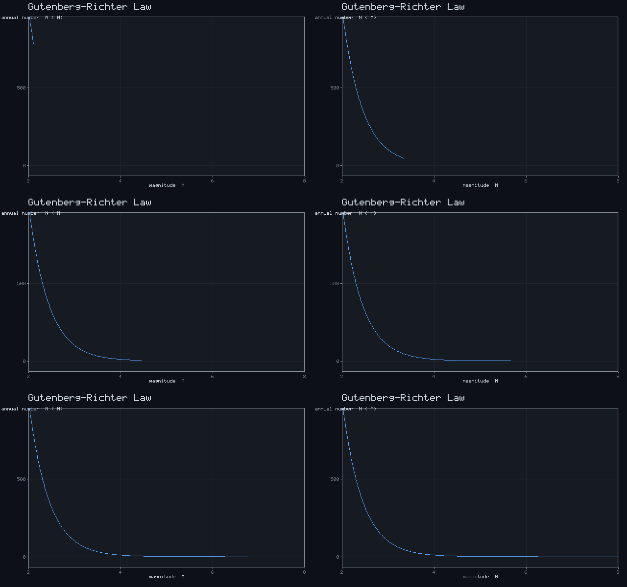

Gutenberg-Richter Law

log₁₀ N = a − b·M (a=5, b=1)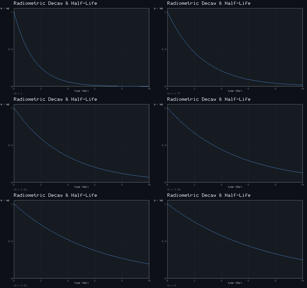

Radiometric Decay & Half-Life

N = N₀·e^(−λt), λ = ln2 / t½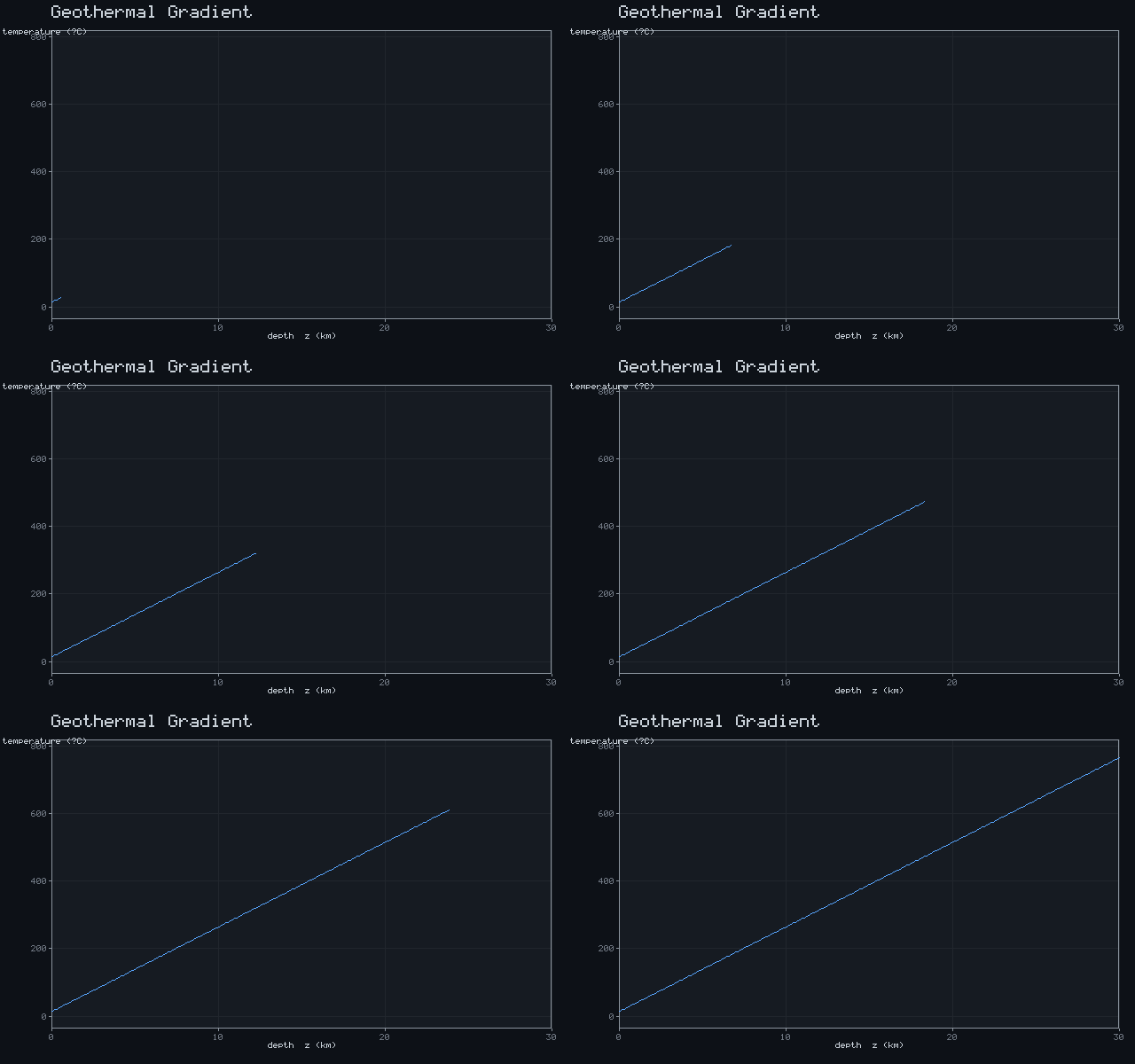

Geothermal Gradient

T = T₀ + G·z (G ≈ 25 °C/km)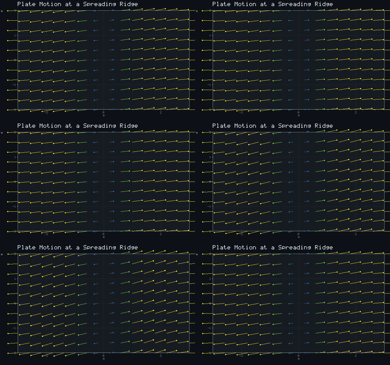

Plate Motion at a Spreading Ridge

v(x) diverging from the ridge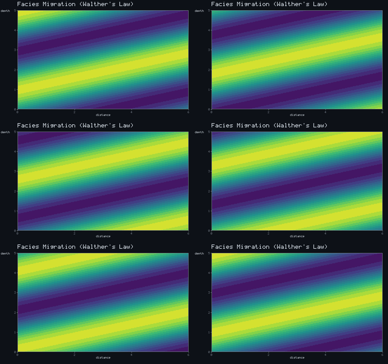

Facies Migration (Walther's Law)

shoreline transgression / regression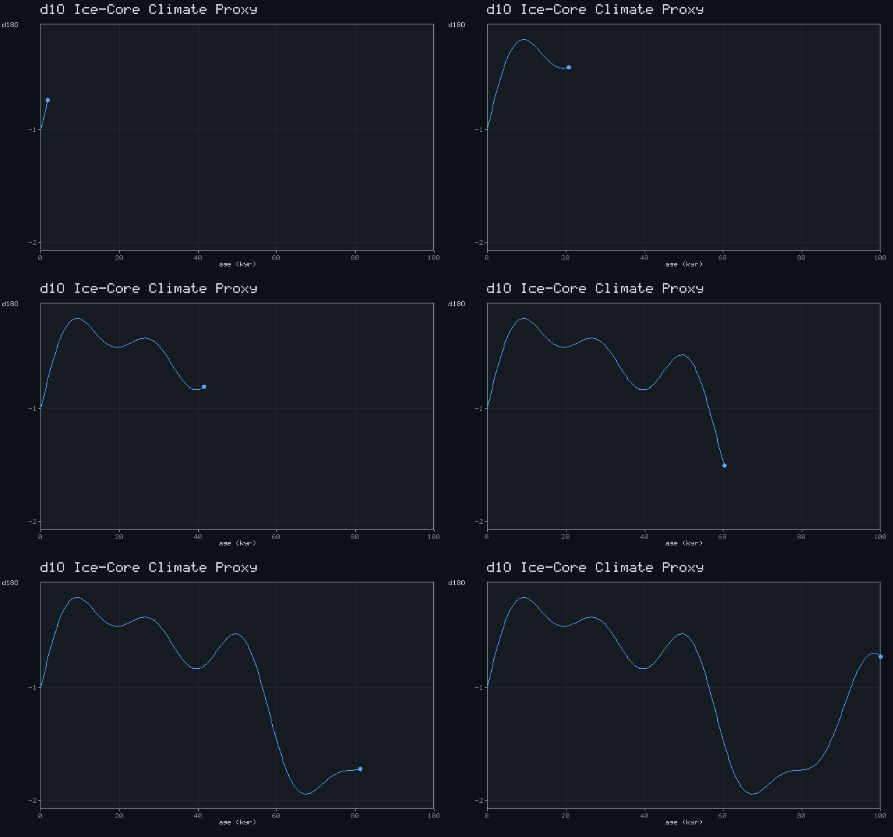

δ¹⁸O Ice-Core Climate Proxy

Milankovitch 100 / 41 / 23 kyr cycles

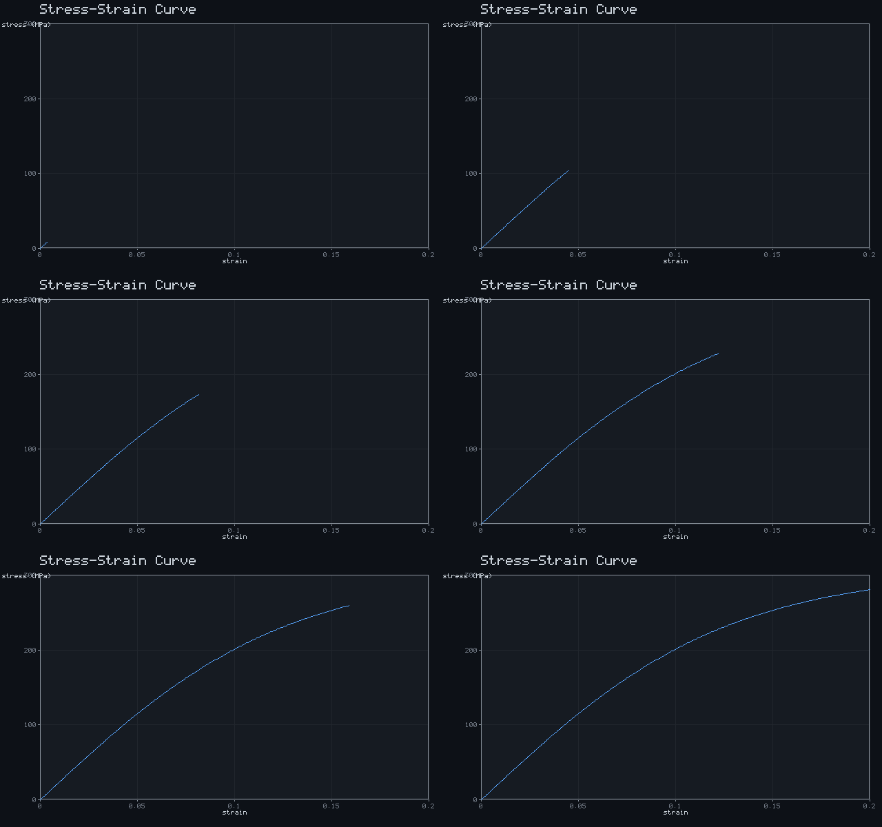
Stress-Strain Curve

σ = 300·tanh(8ε) + 20ε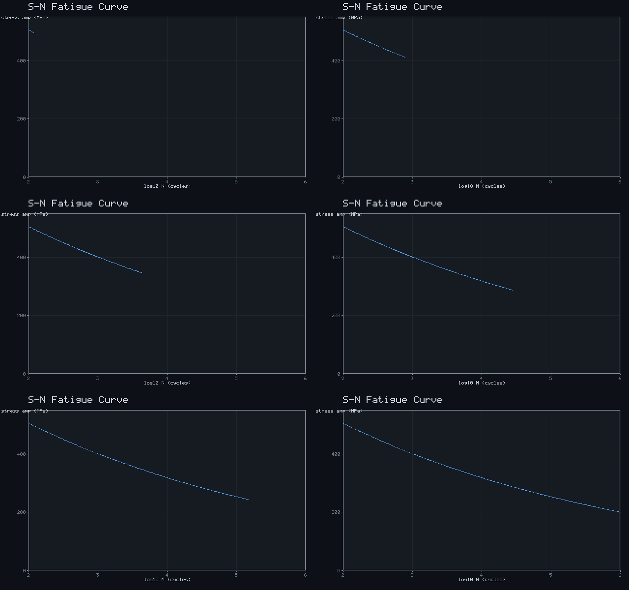

S-N Fatigue Curve

S = C·N^(-0.1) (Basquin)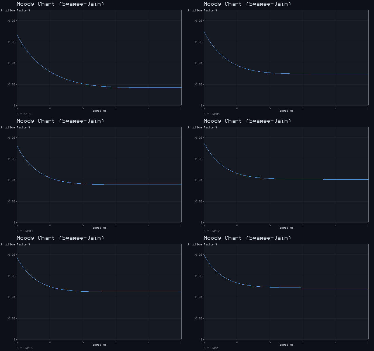

Moody Chart (Swamee-Jain)

f = 0.25 / log₁₀(ε/3.7 + 5.74/Re^0.9)²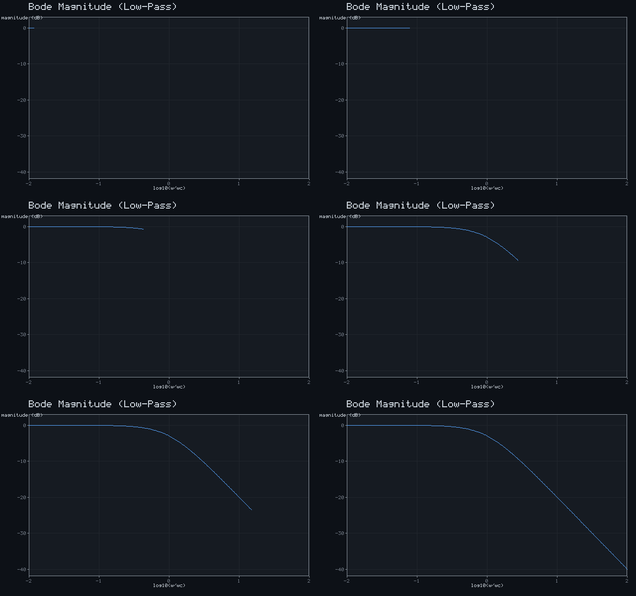

Bode Magnitude (Low-Pass)

|H| = -10·log₁₀(1 + (ω/ω_c)²) dB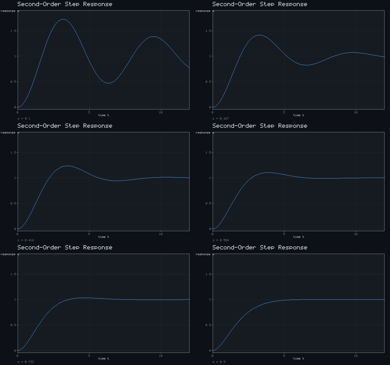

Second-Order Step Response

y = 1 − e^(−ζt)·(cos ω_d t + ζ/ω_d · sin ω_d t)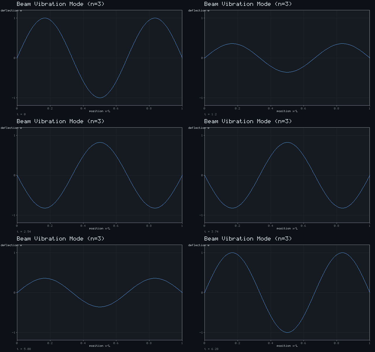

Beam Vibration Mode (n=3)

w(x,t) = sin(3πx/L)·cos(ωt)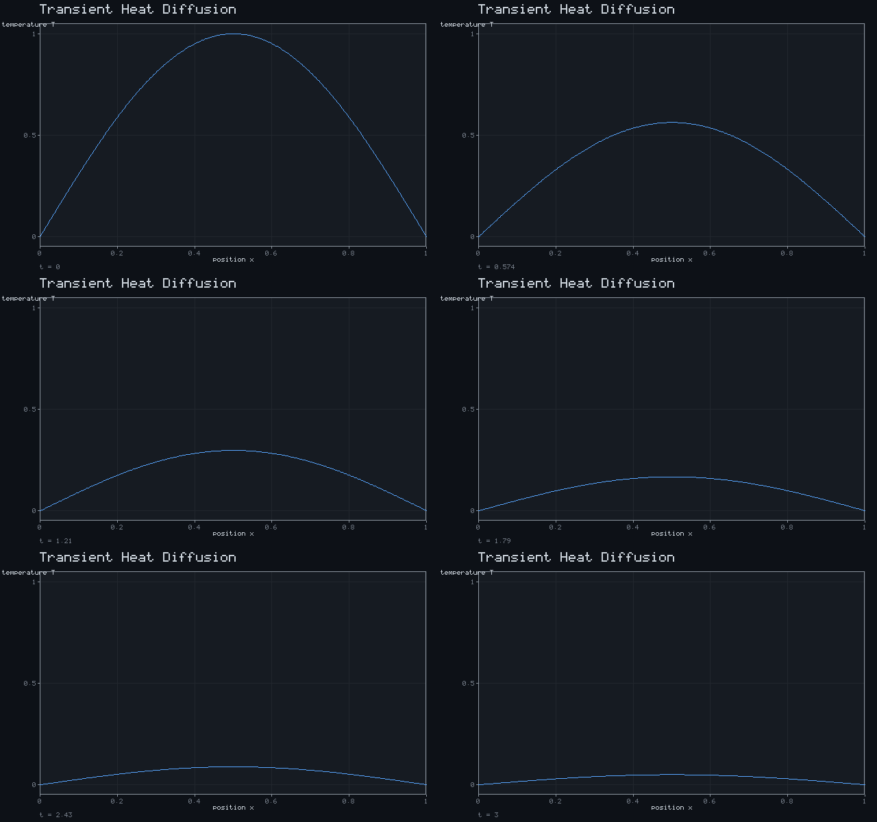

Transient Heat Diffusion

T(x,t) = e^(−t)·sin(πx)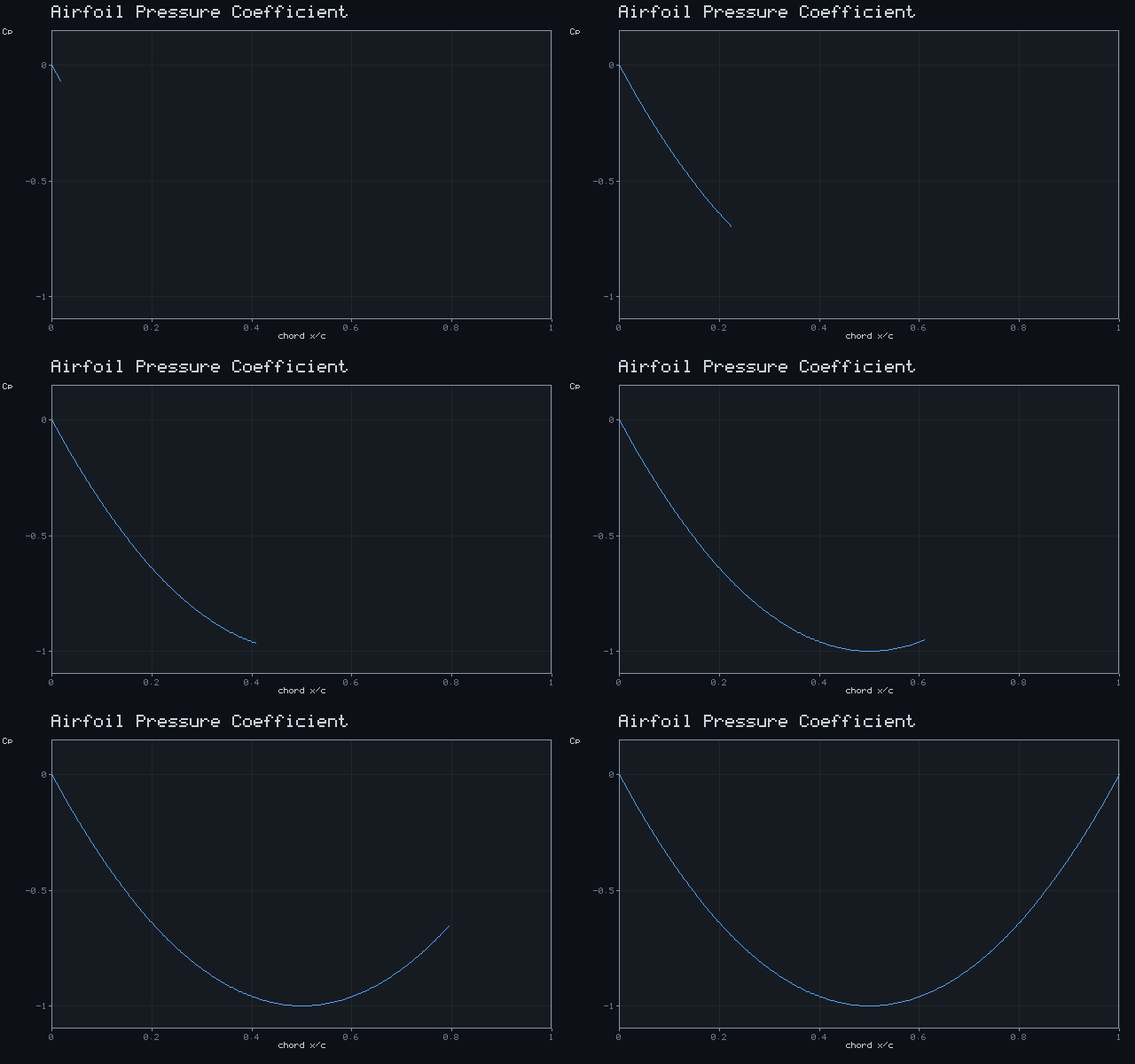

Airfoil Pressure Coefficient

C_p ≈ −4·(x/c)·(1 − x/c)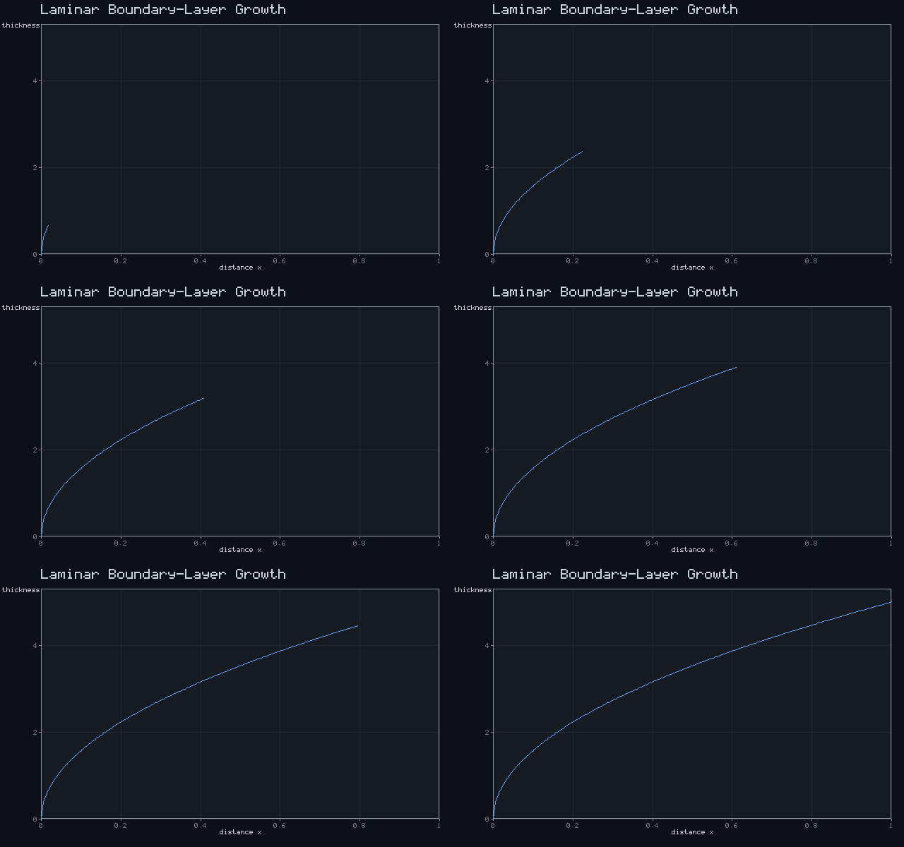

Laminar Boundary-Layer Growth

δ ∝ √x (Blasius)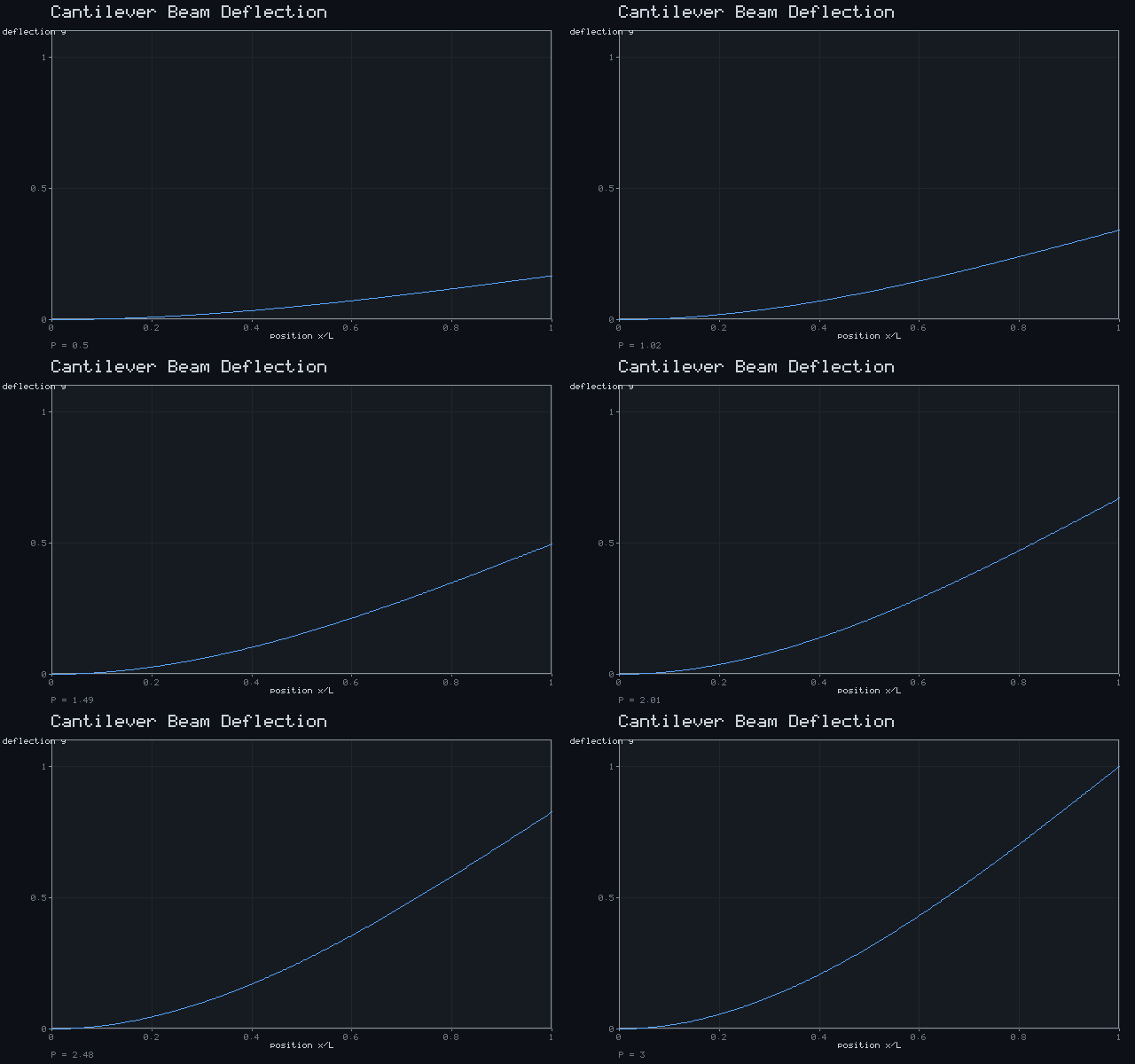

Cantilever Beam Deflection

y = P·x²·(3L − x) / 6EI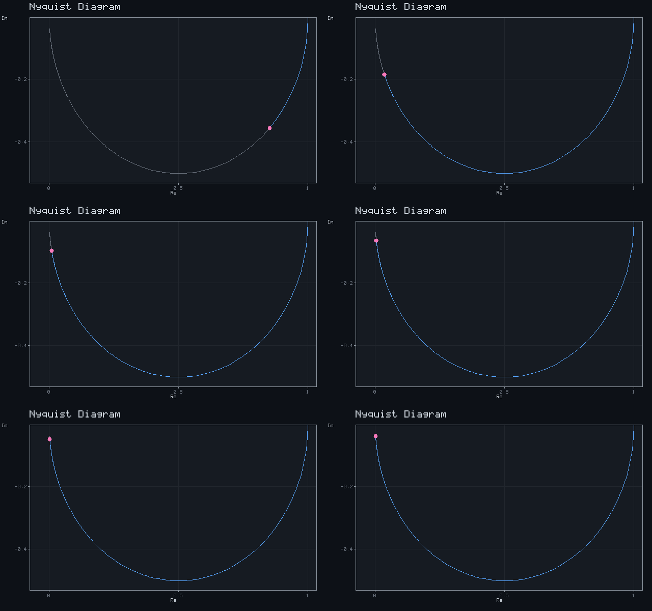

Nyquist Diagram

G(iω) = 1 / (1 + iω)

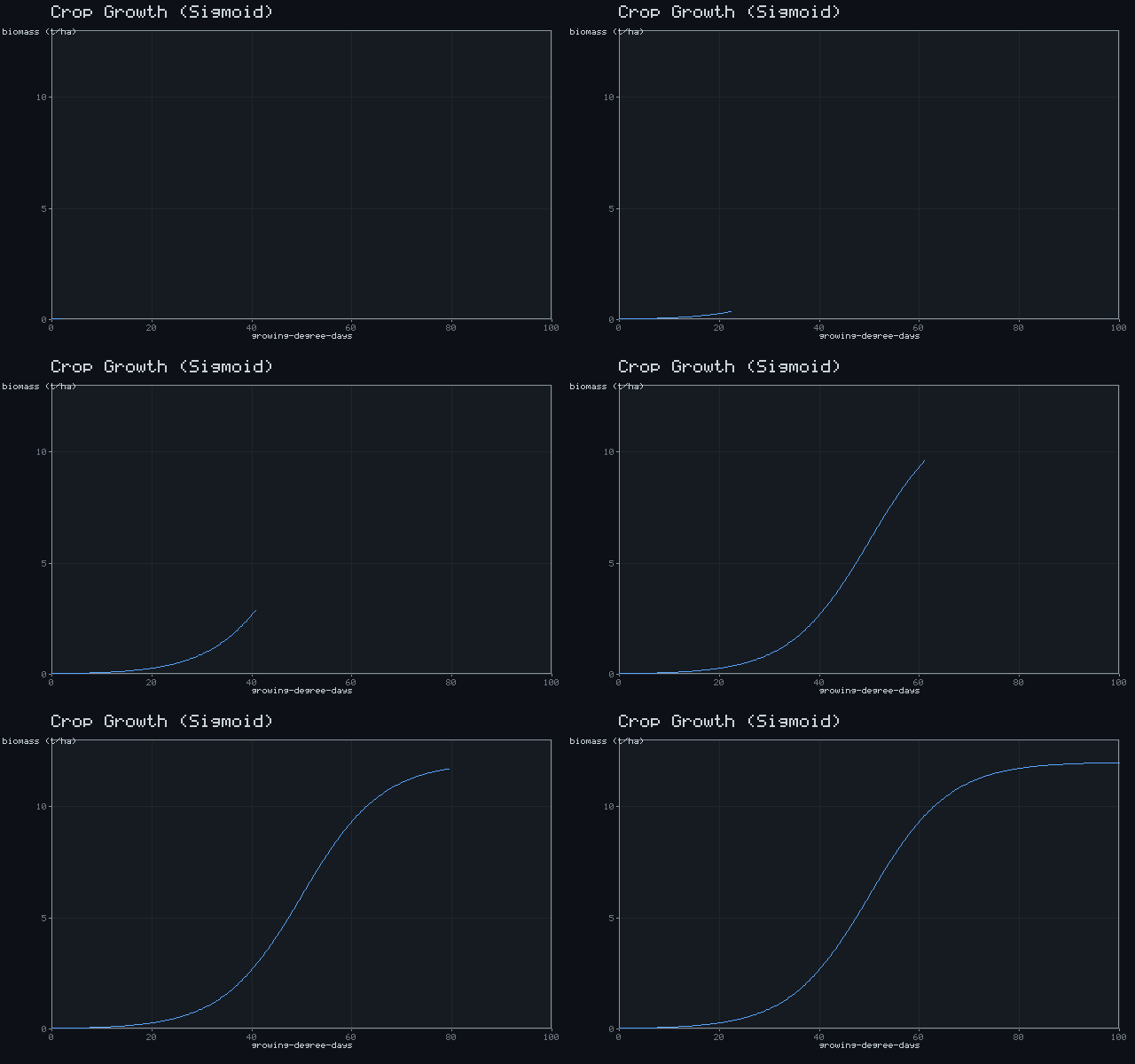
Crop Growth (Sigmoid)

B = Bmax / (1 + e^(-(GDD-50)/8))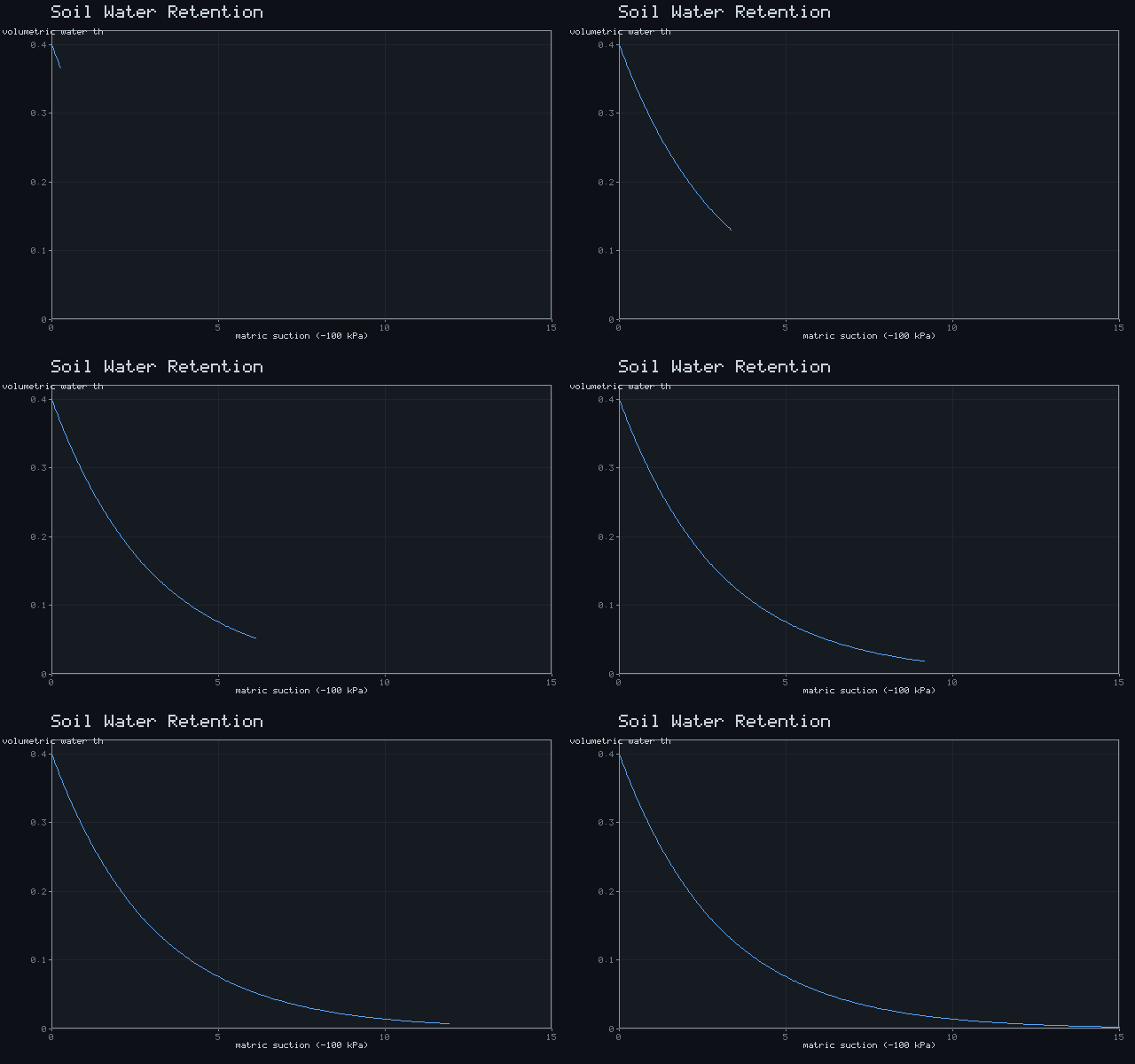

Soil Water Retention

θ = θs · e^(-ψ/α)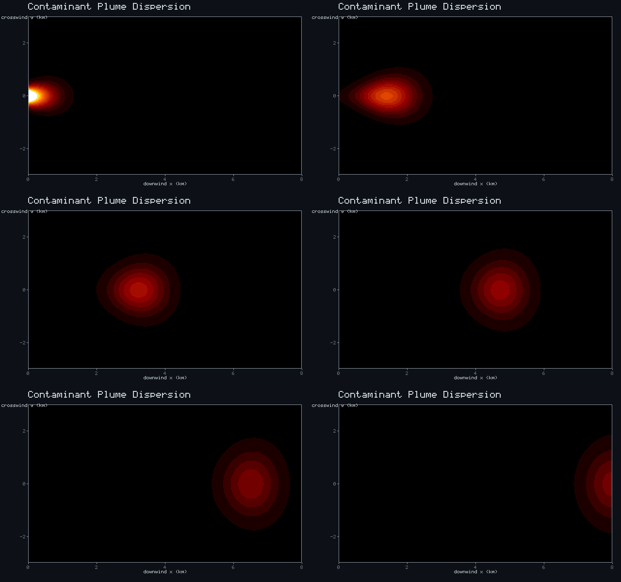

Contaminant Plume Dispersion

C(x,y) = e^(-y²/(2σ²(x))) / √x · puff(x-ut)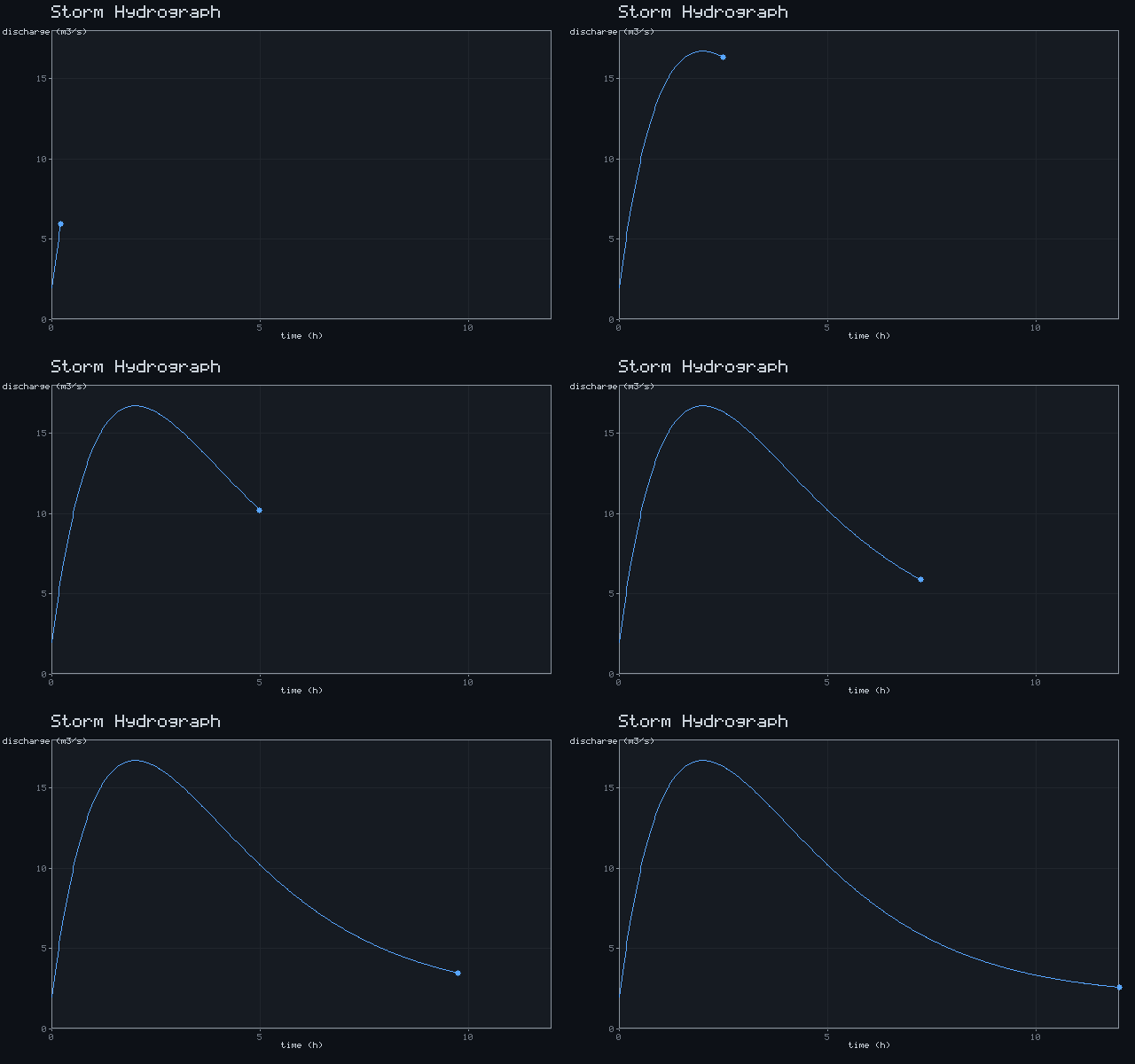

Storm Hydrograph

Q(t) = Qb + a·t·e^(-t/b)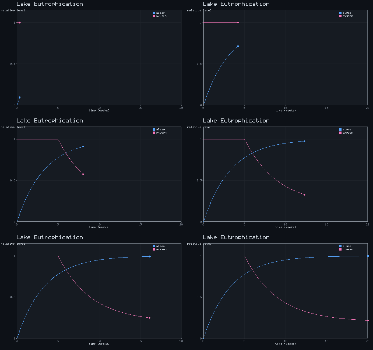

Lake Eutrophication

algae ↑ then dissolved O₂ crash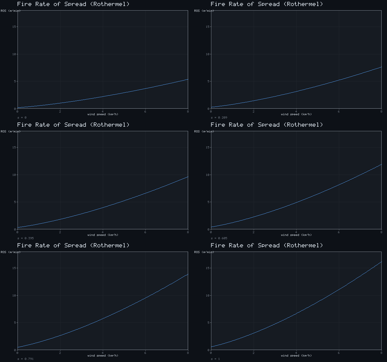

Fire Rate of Spread (Rothermel)

R = R0·(1+U)^1.5·(1+2·φs)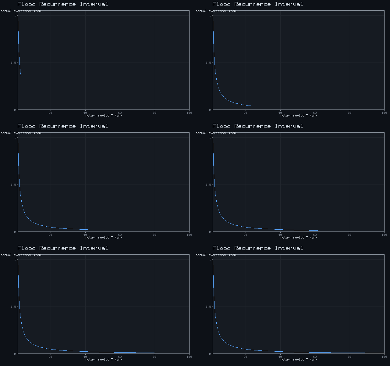

Flood Recurrence Interval

P = 1 / T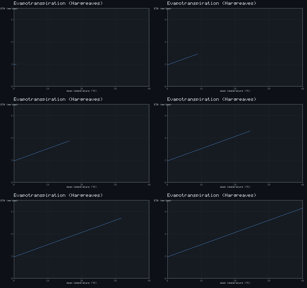

Evapotranspiration (Hargreaves)

ET0 = 0.0023·Ra·(T+17.8)·√ΔT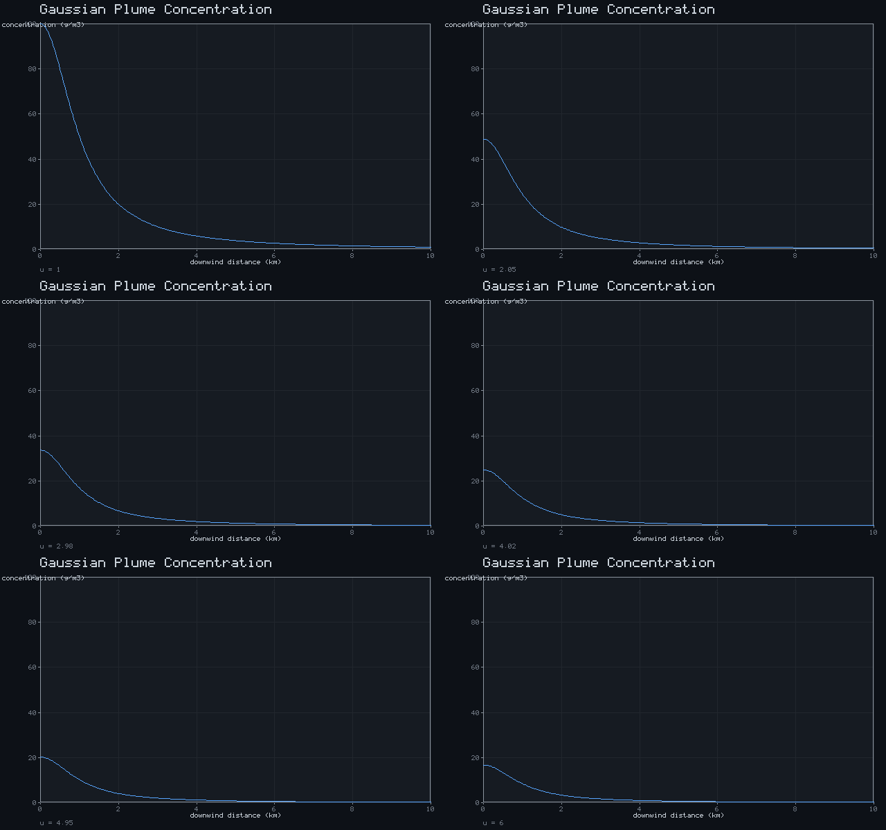

Gaussian Plume Concentration

C(x) = Q / (u·(x²+1))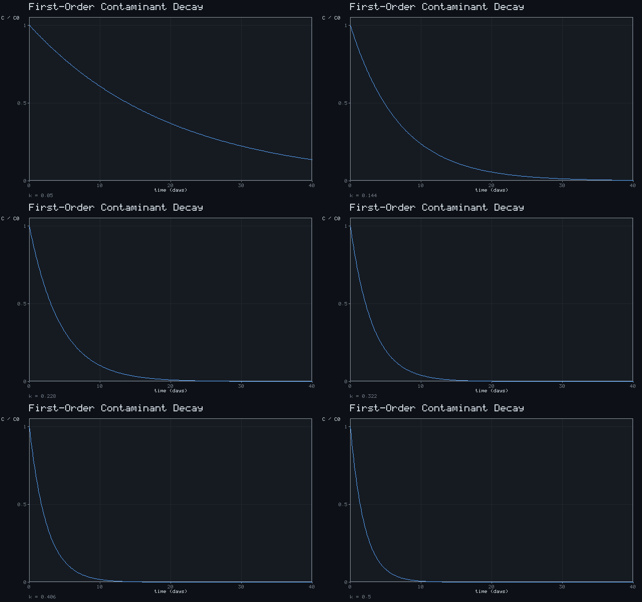

First-Order Contaminant Decay

C = C0 · e^(-k·t)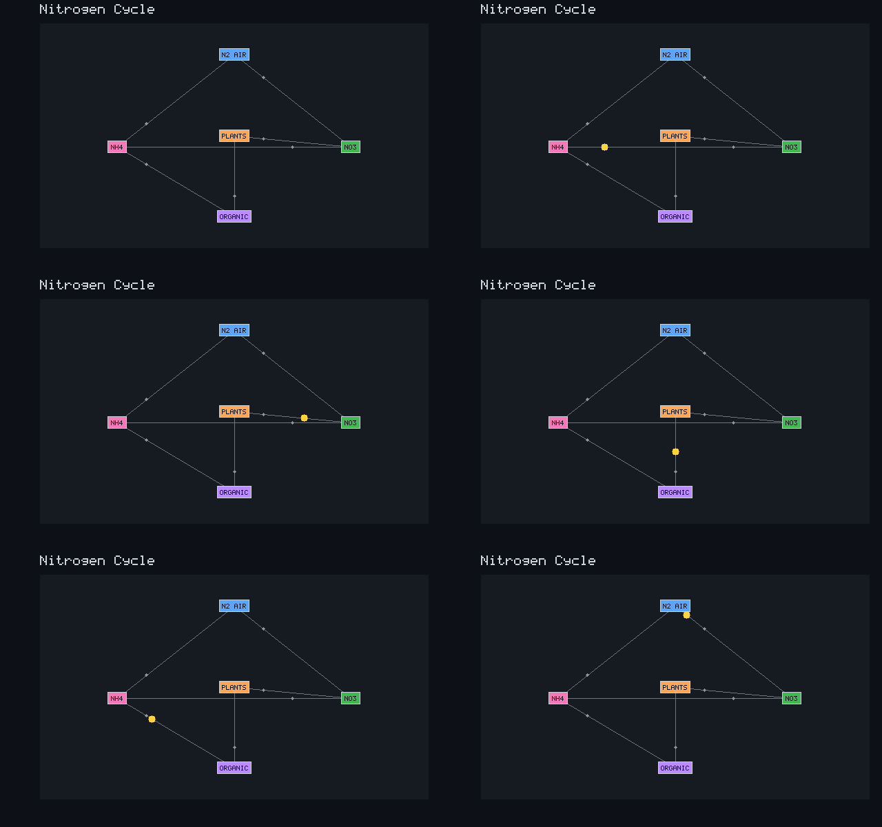

Nitrogen Cycle

fixation → nitrification → uptake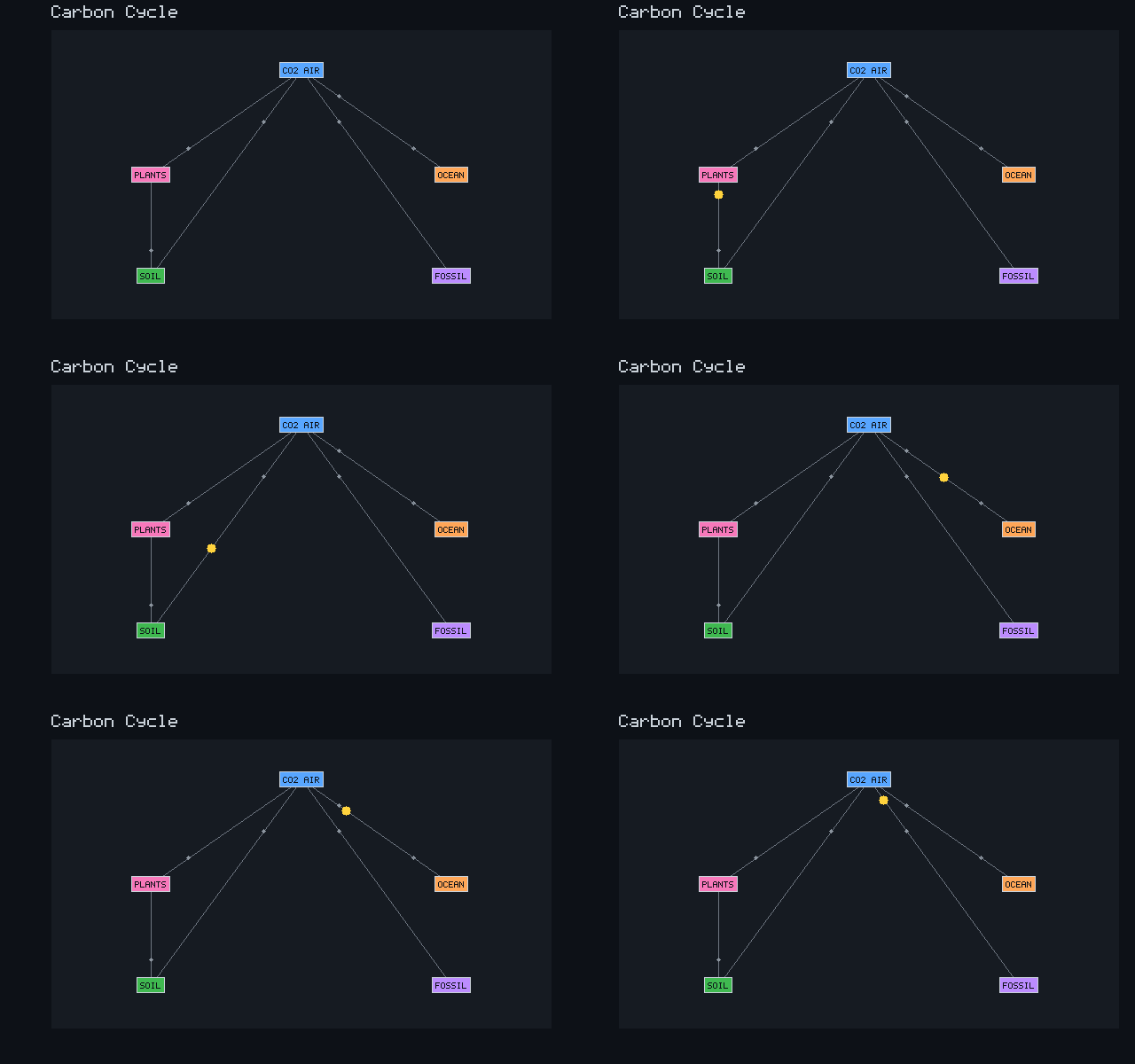

Carbon Cycle

photosynthesis ⇌ respiration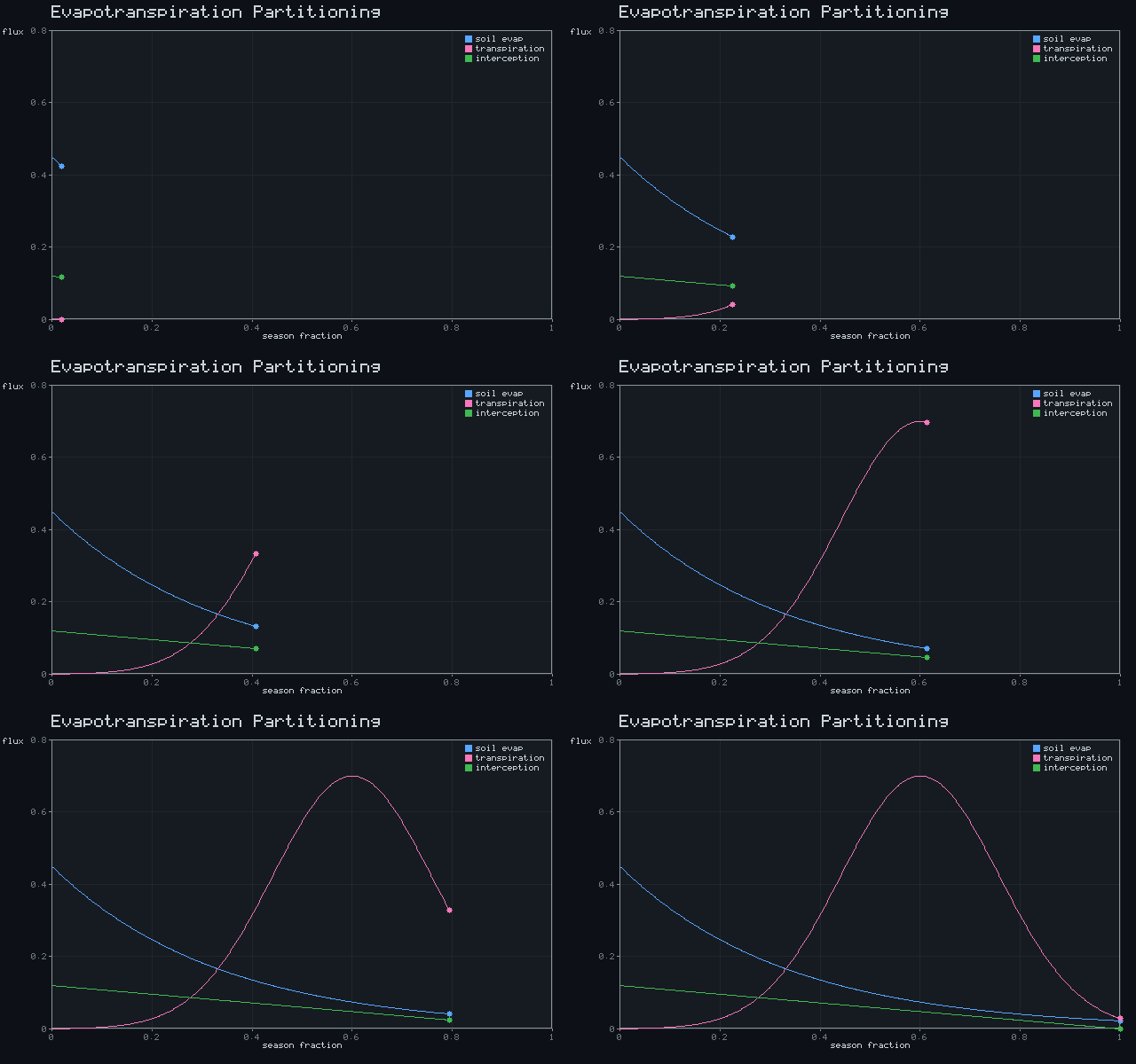

Evapotranspiration Partitioning

ET = E_soil + T_plant + I_canopy

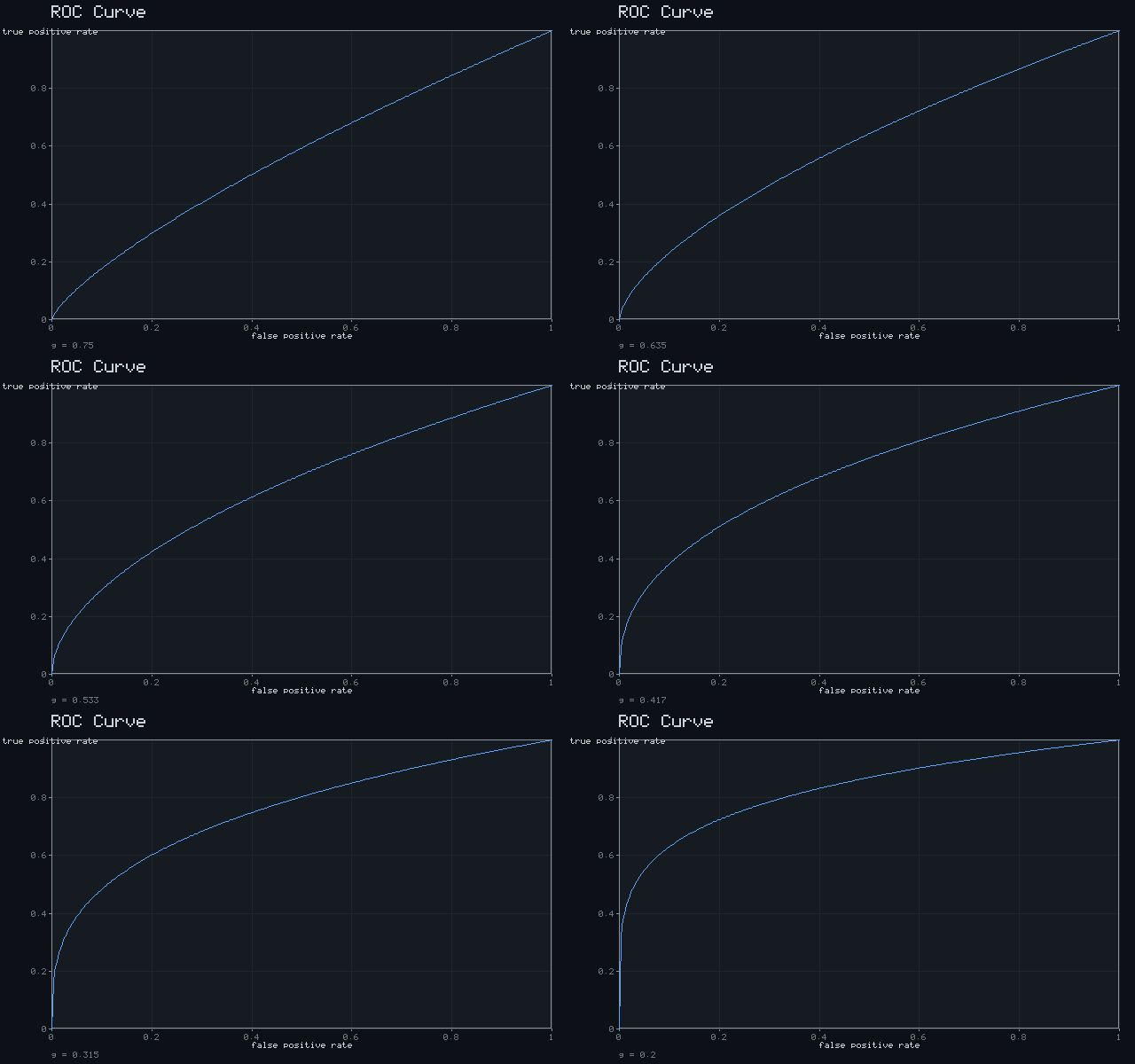
ROC Curve

TPR = FPR^γ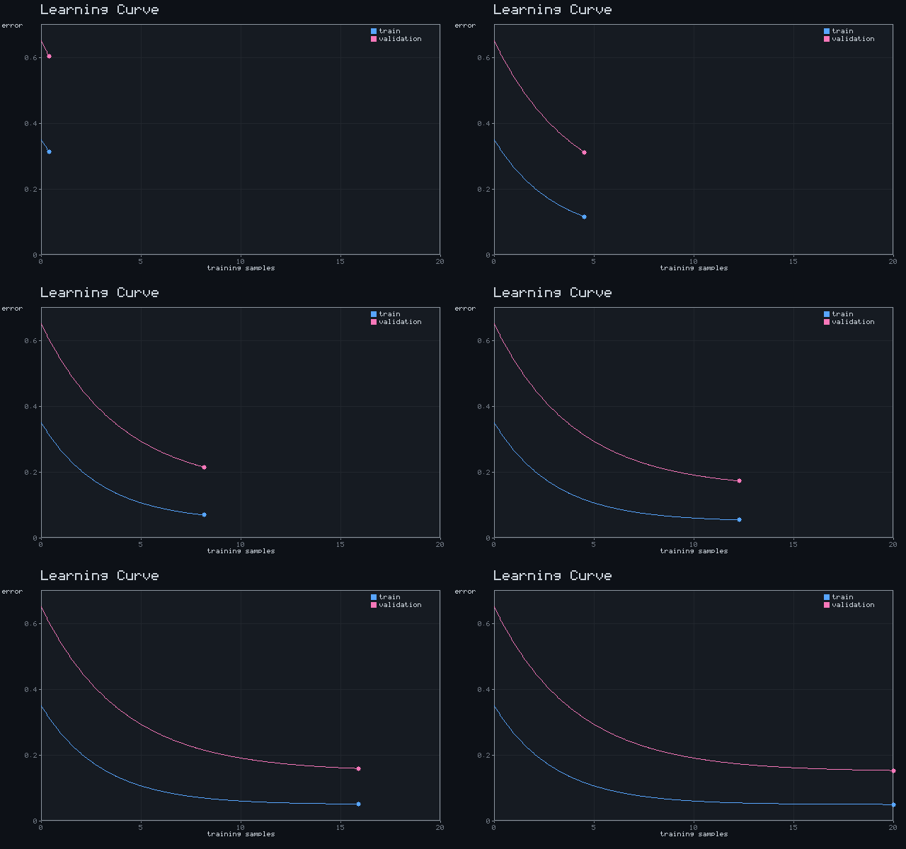

Learning Curve

E(n) = a + b·e^(−n/τ)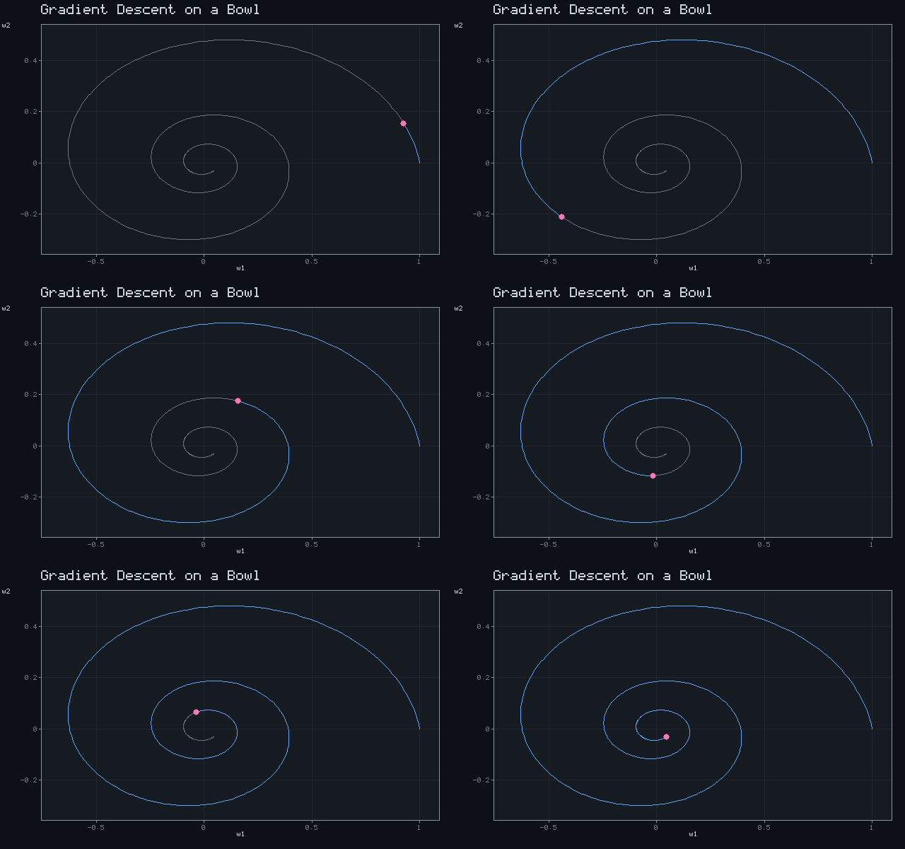

Gradient Descent on a Bowl

θ ← θ − η∇J(θ)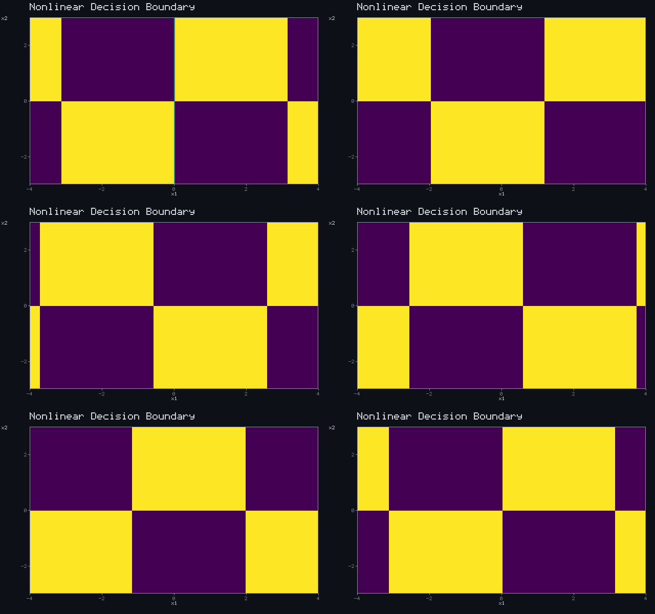

Nonlinear Decision Boundary

ŷ = sign(sin x · sin y)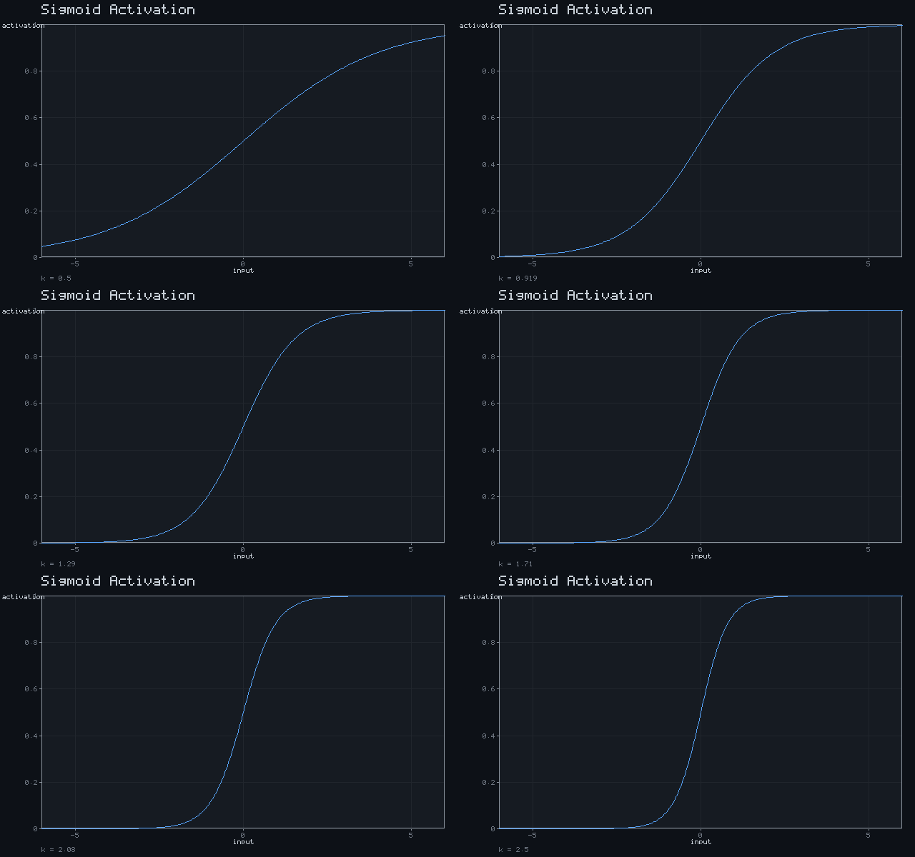

Sigmoid Activation

σ(x) = 1 / (1 + e^(−kx))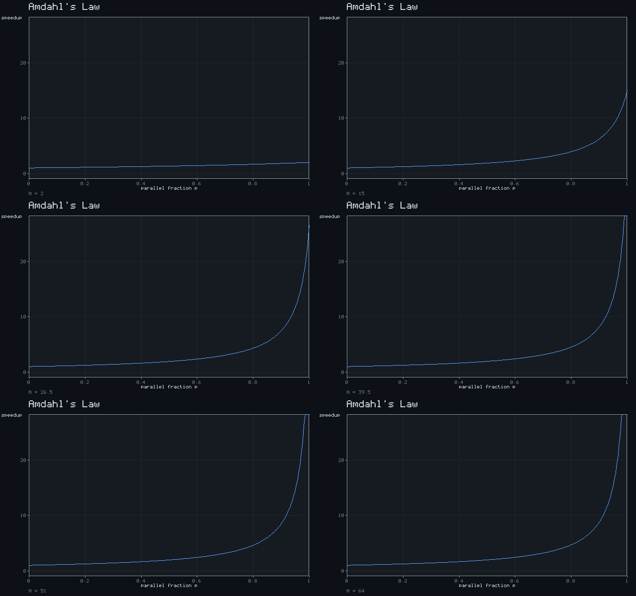

Amdahl's Law

S = 1 / ((1−p) + p/N)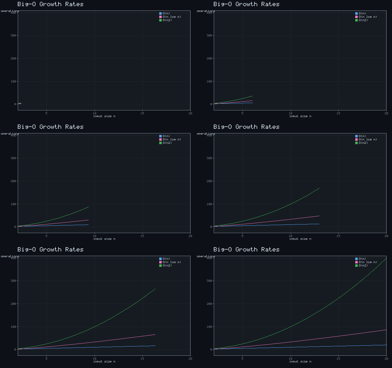

Big-O Growth Rates

T(n) ∈ {n, n log₂n, n²}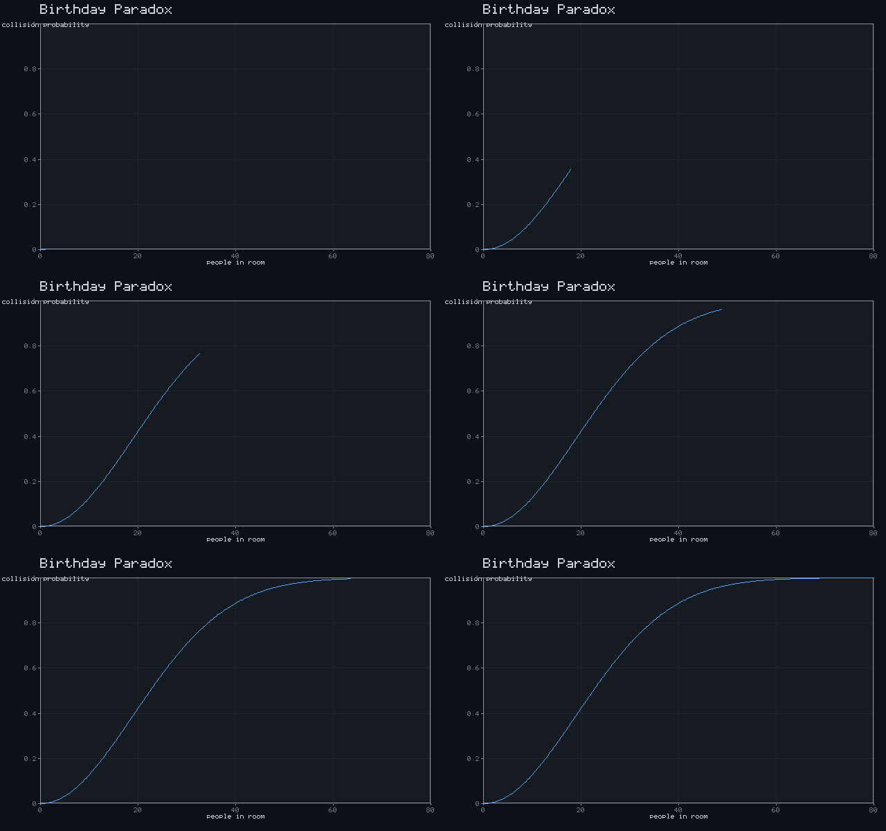

Birthday Paradox

P = 1 − e^(−n²/730)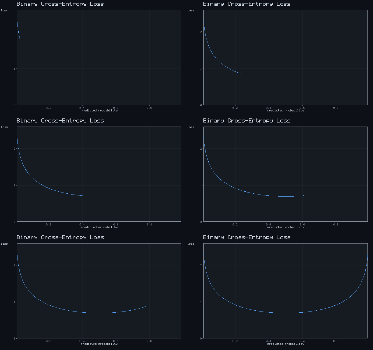

Binary Cross-Entropy Loss

L = −[y ln p + (1−y) ln(1−p)]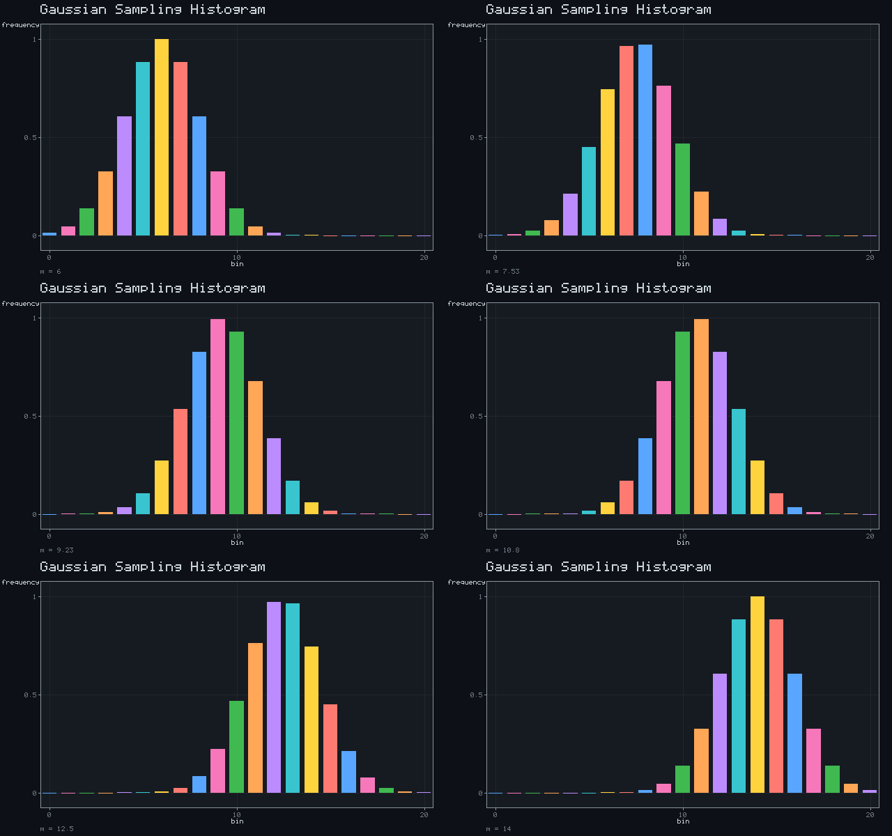

Gaussian Sampling Histogram

f(x) = e^(−(x−μ)²/8)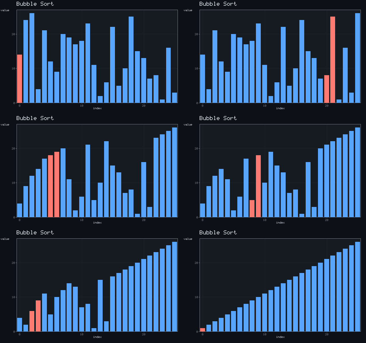

Bubble Sort

compare-and-swap adjacent pairs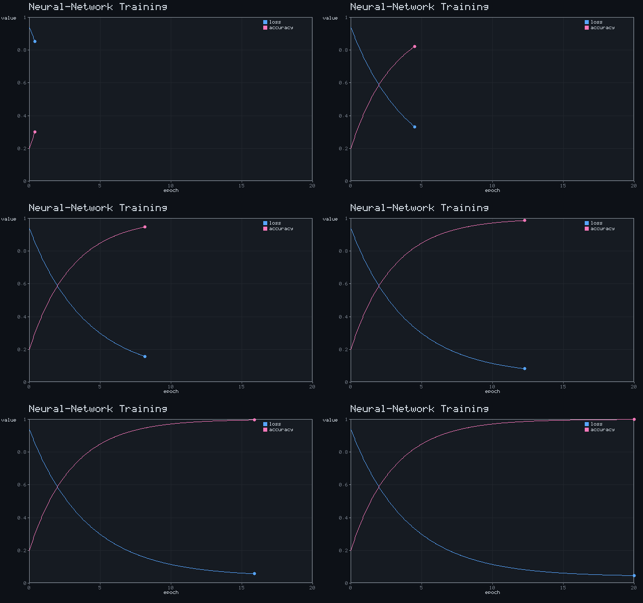

Neural-Network Training

loss ↓, accuracy ↑ over epochs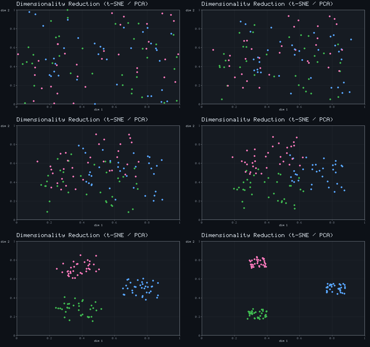

Dimensionality Reduction (t-SNE / PCA)

high-D → 2-D embedding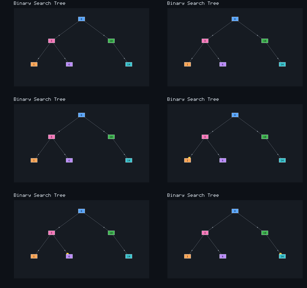

Binary Search Tree

left < node < right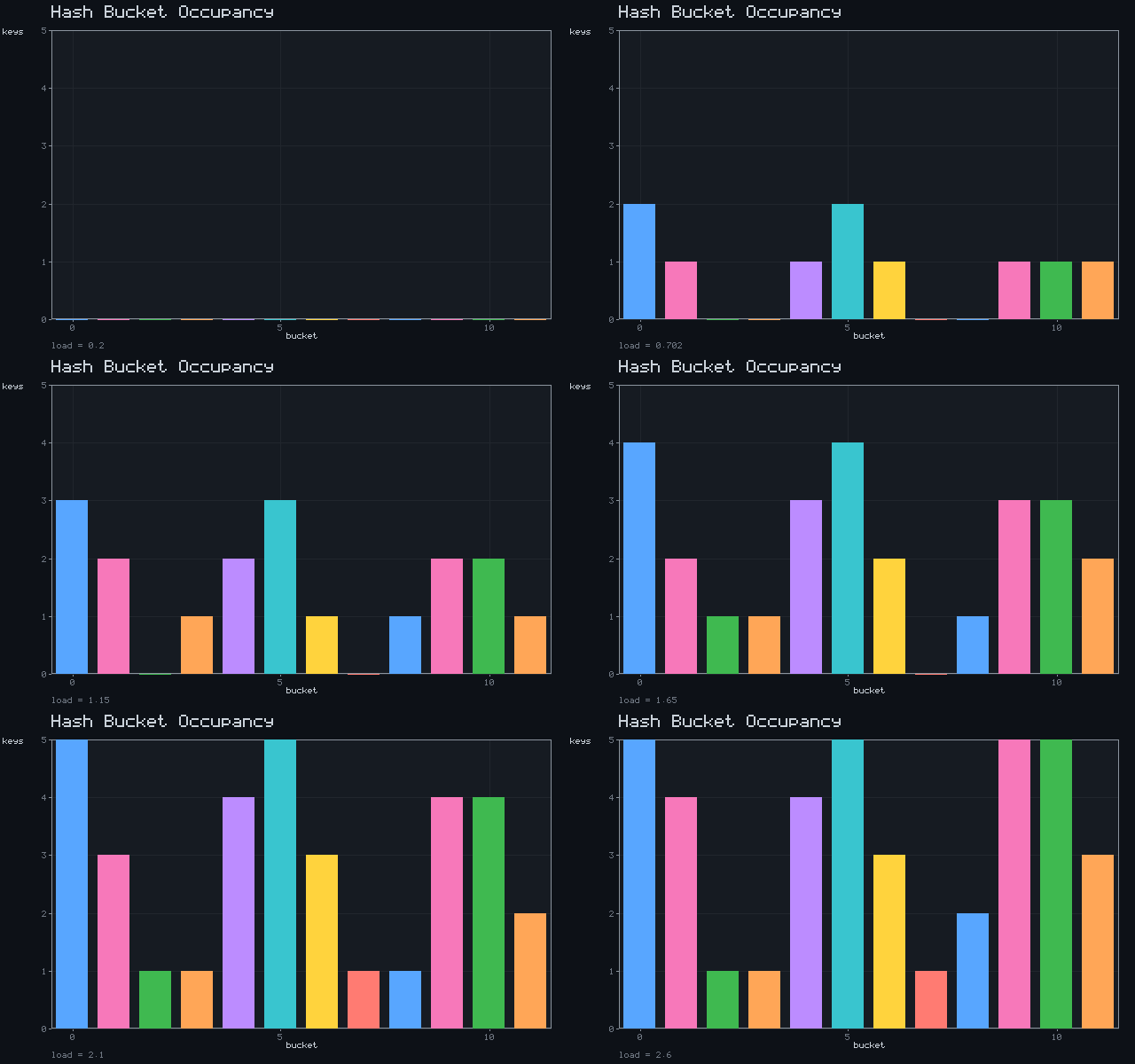

Hash Bucket Occupancy

collisions rise with load factor α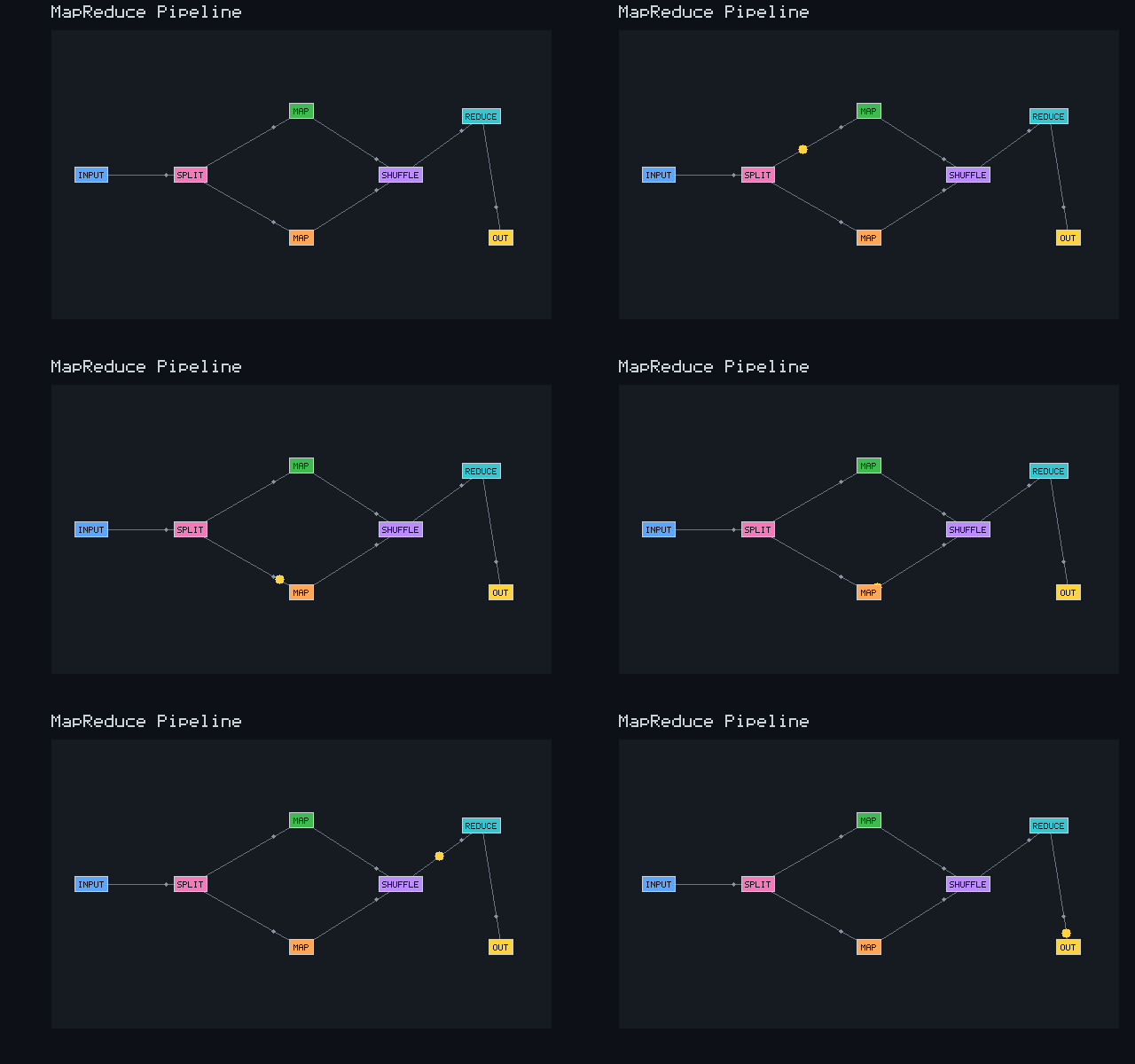

MapReduce Pipeline

split → map → shuffle → reduce

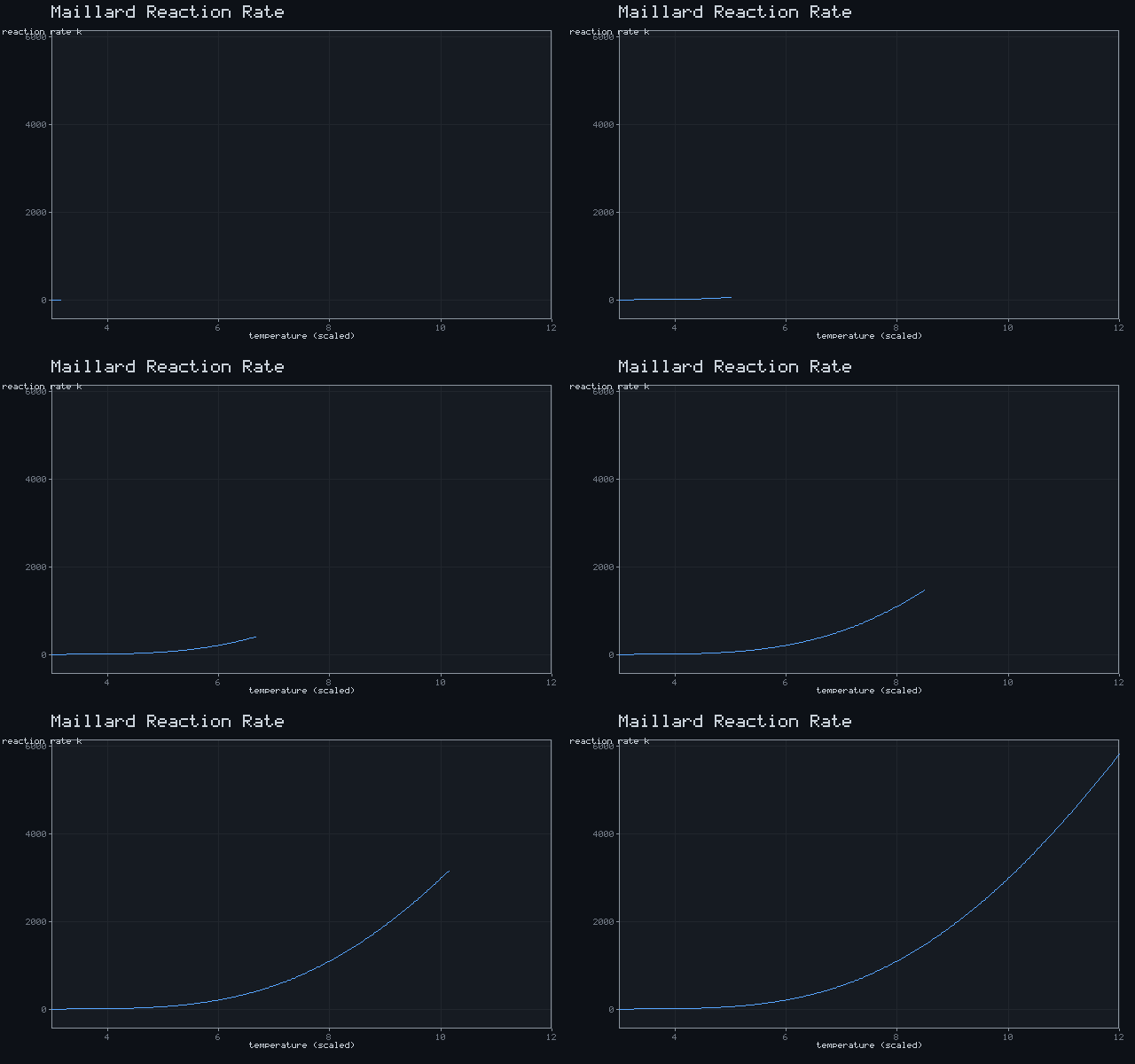
Maillard Reaction Rate

k ∝ exp(12 − 40/T)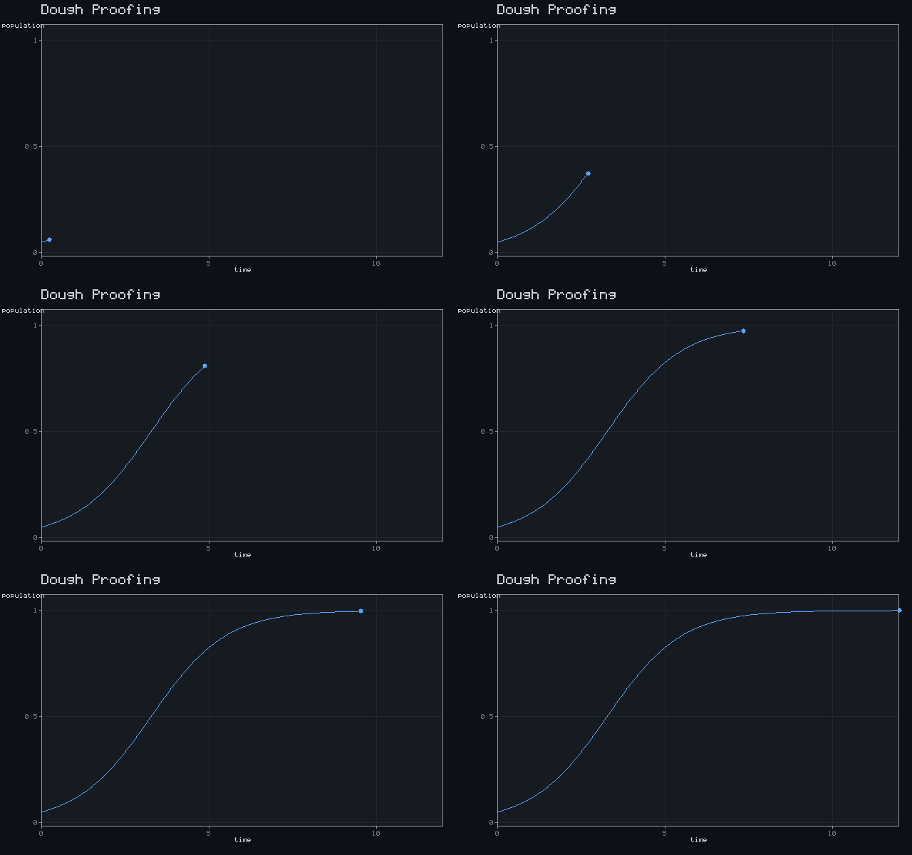

Dough Proofing

dN/dt = r·N·(1 − N/K)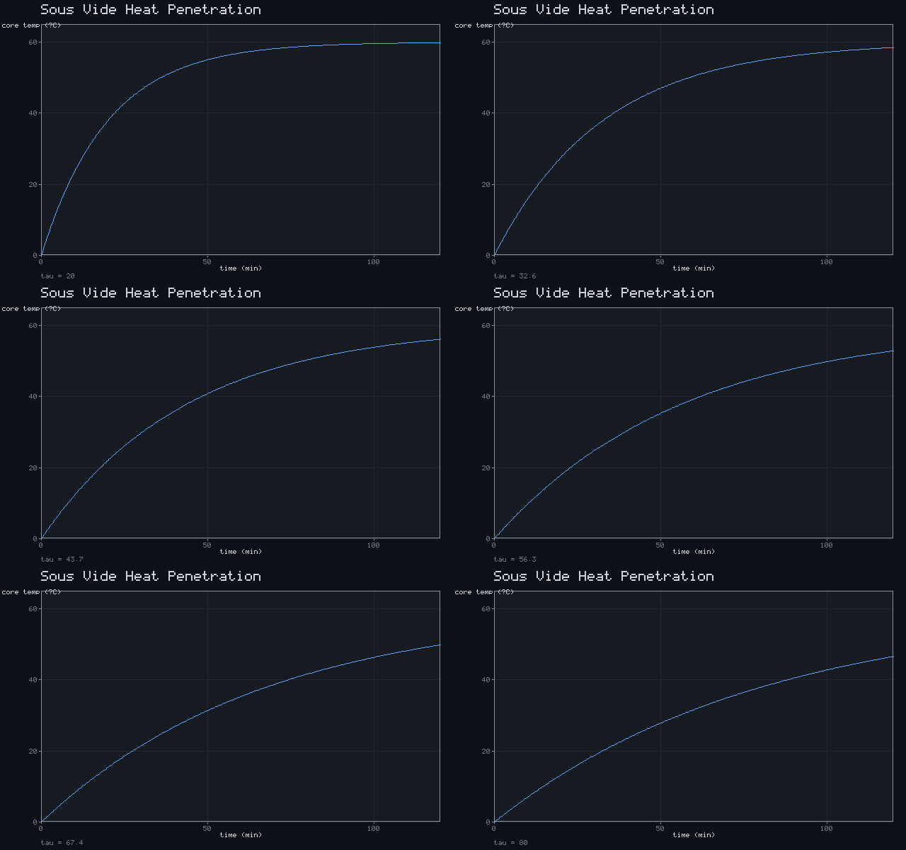

Sous Vide Heat Penetration

T = 60·(1 − e^(−t/τ))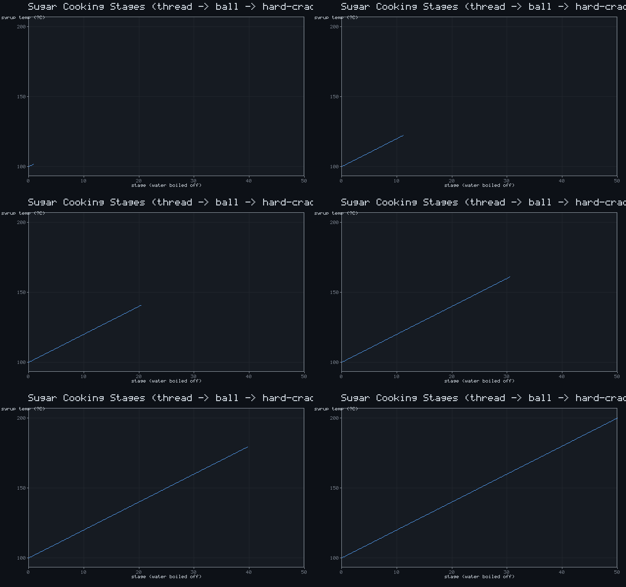

Sugar Cooking Stages (thread → ball → hard-crack)

T ≈ 100 + 2·s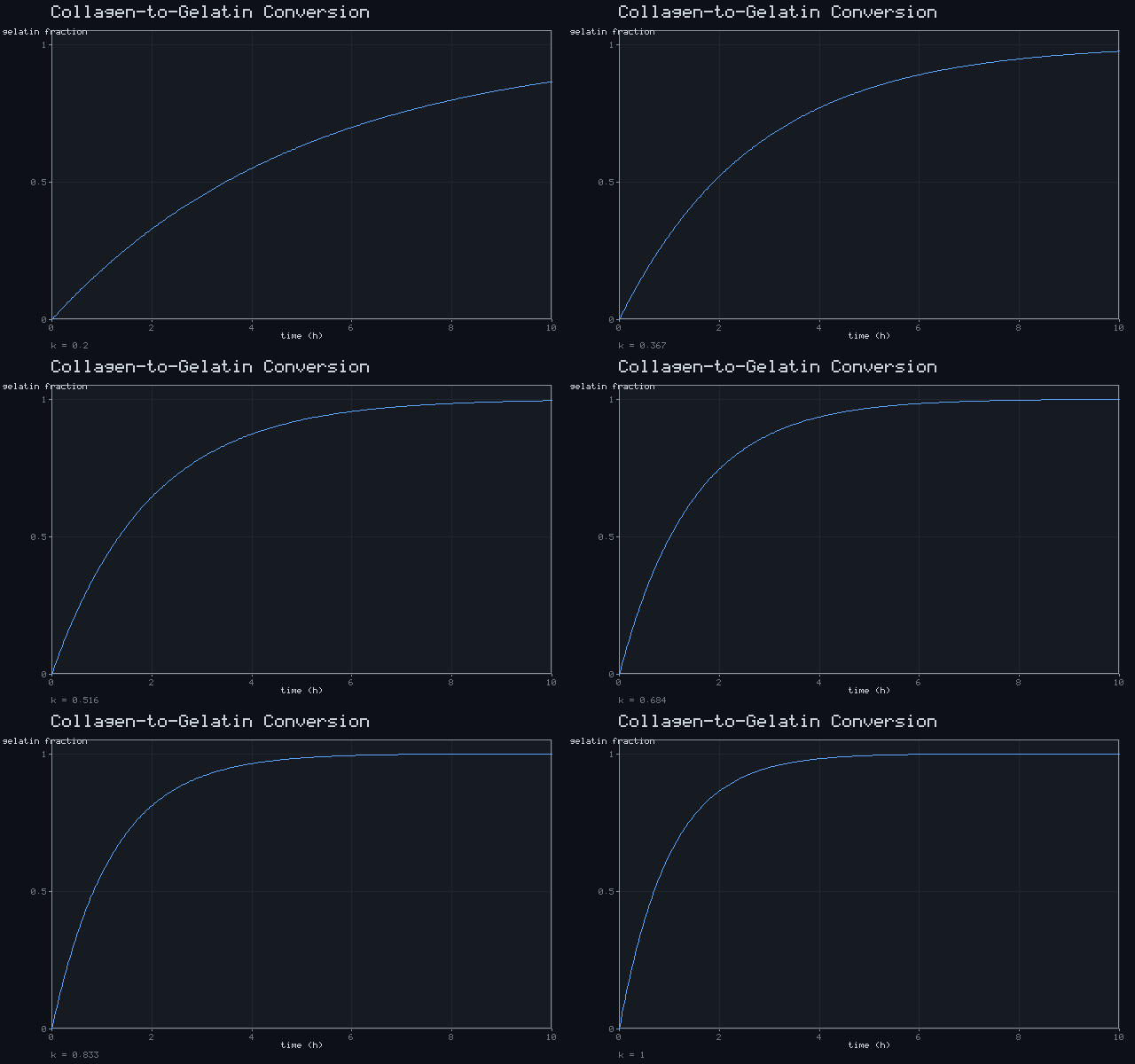

Collagen-to-Gelatin Conversion

f = 1 − e^(−k·t)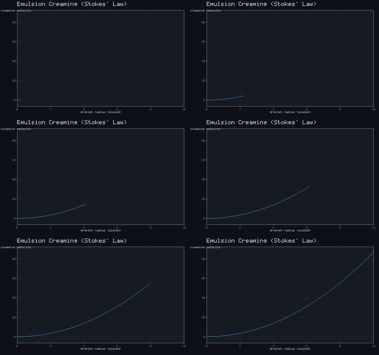

Emulsion Creaming (Stokes' Law)

v = 2·r²·Δρ·g / (9·μ)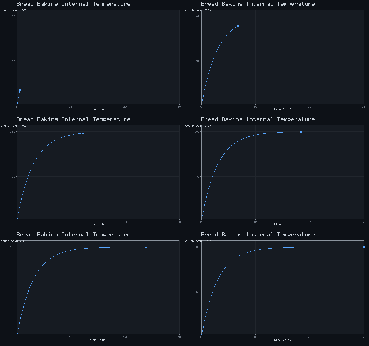

Bread Baking Internal Temperature

T = 100·(1 − e^(−t/3))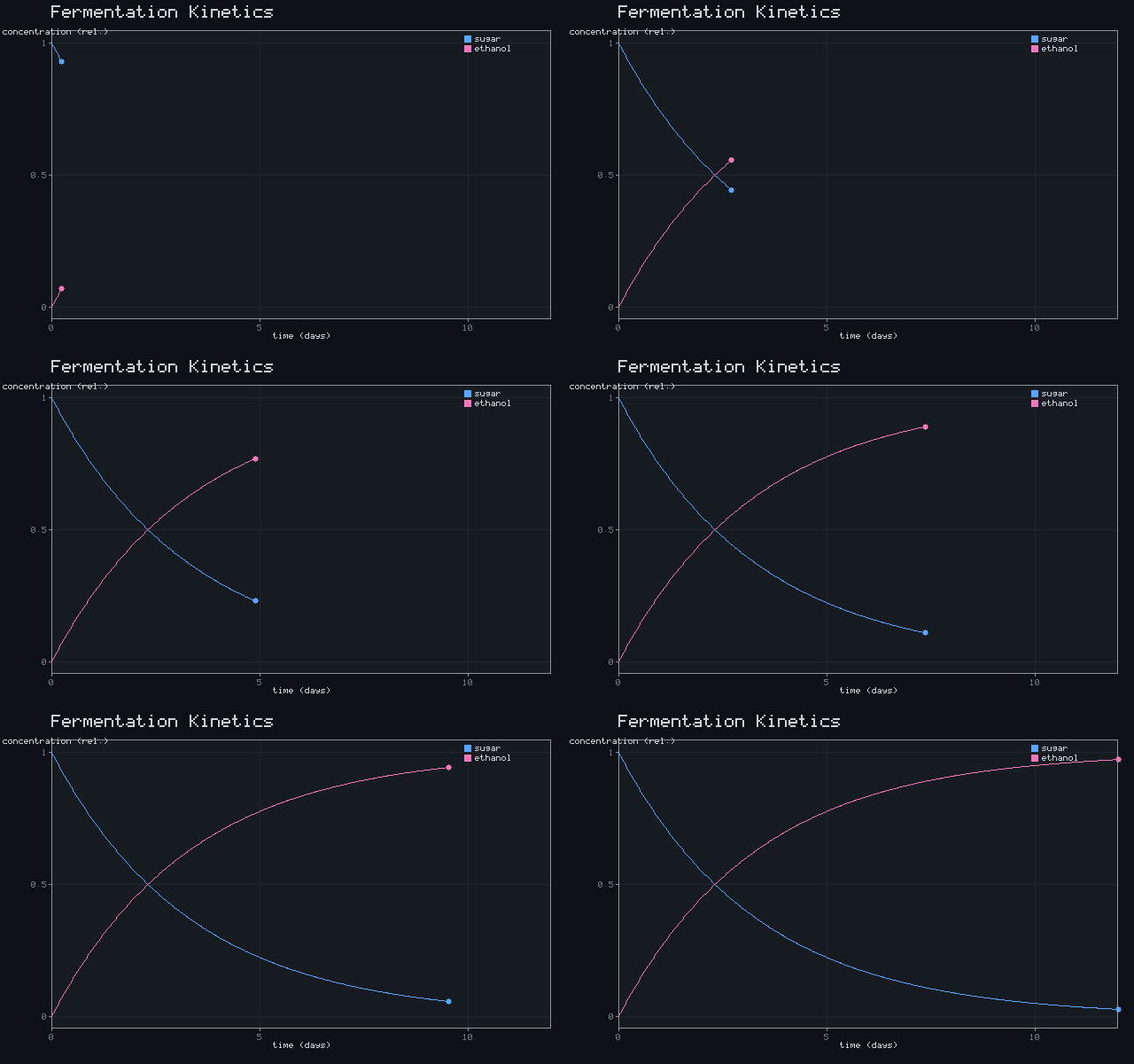

Fermentation Kinetics

S = e^(−0.3t), E = 1 − e^(−0.3t)

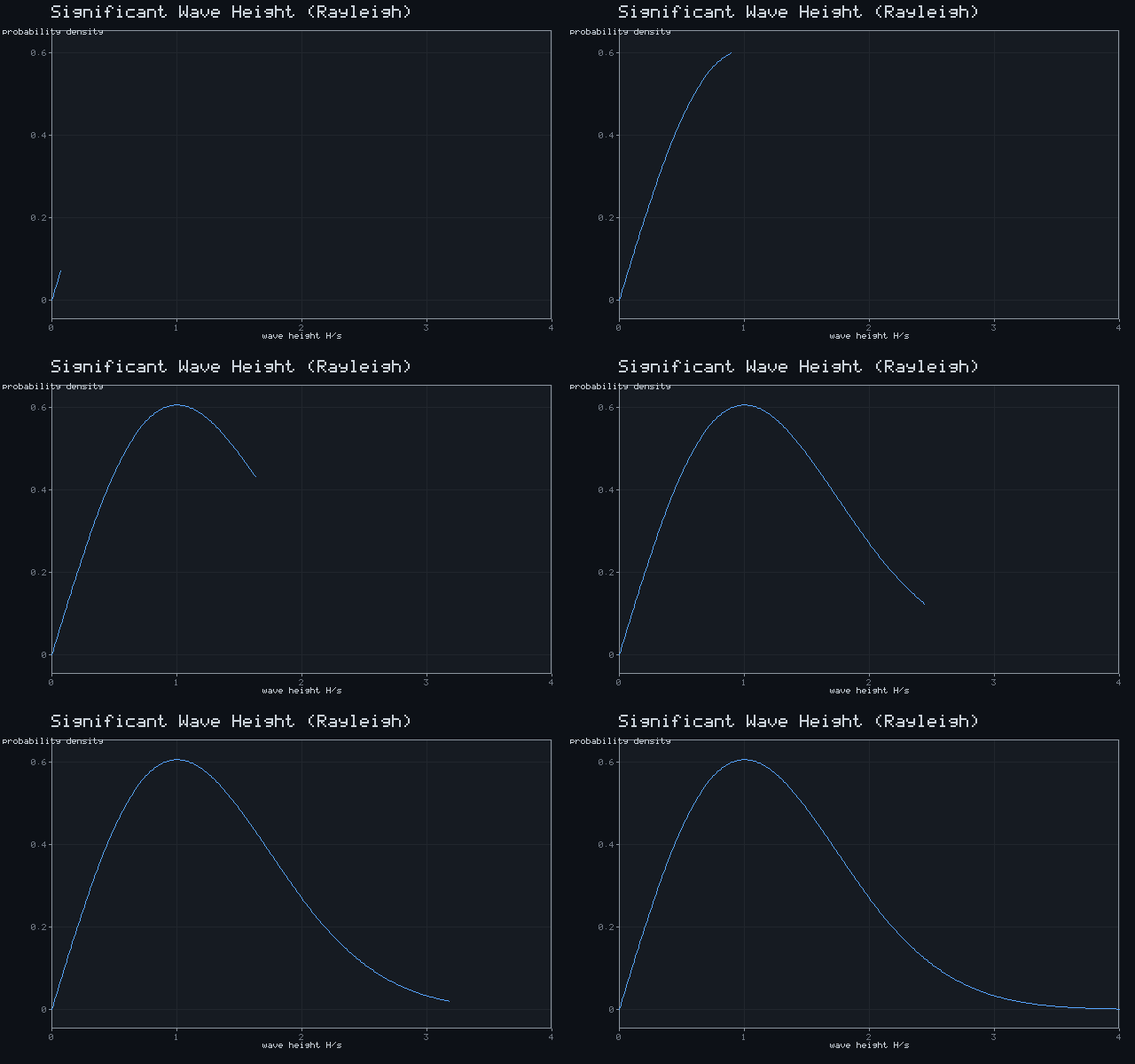
Significant Wave Height (Rayleigh)

p(H) = H·e^(−H²/2)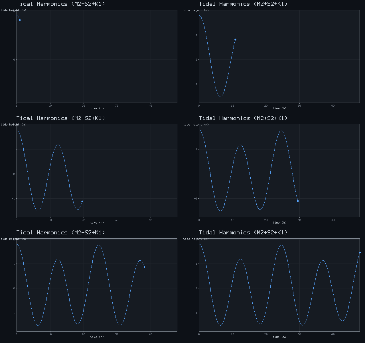

Tidal Harmonics (M₂+S₂+K₁)

η = cos(2πt/12.42) + ½cos(2πt/12) + 0.3cos(2πt/24)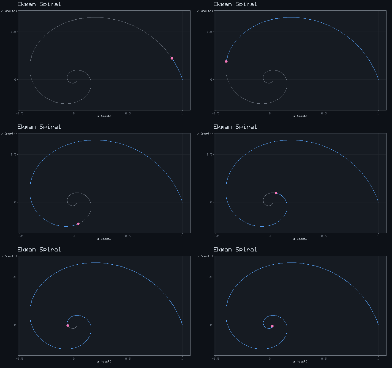

Ekman Spiral

(u,v) = e^(−z/D)·(cos z, sin z)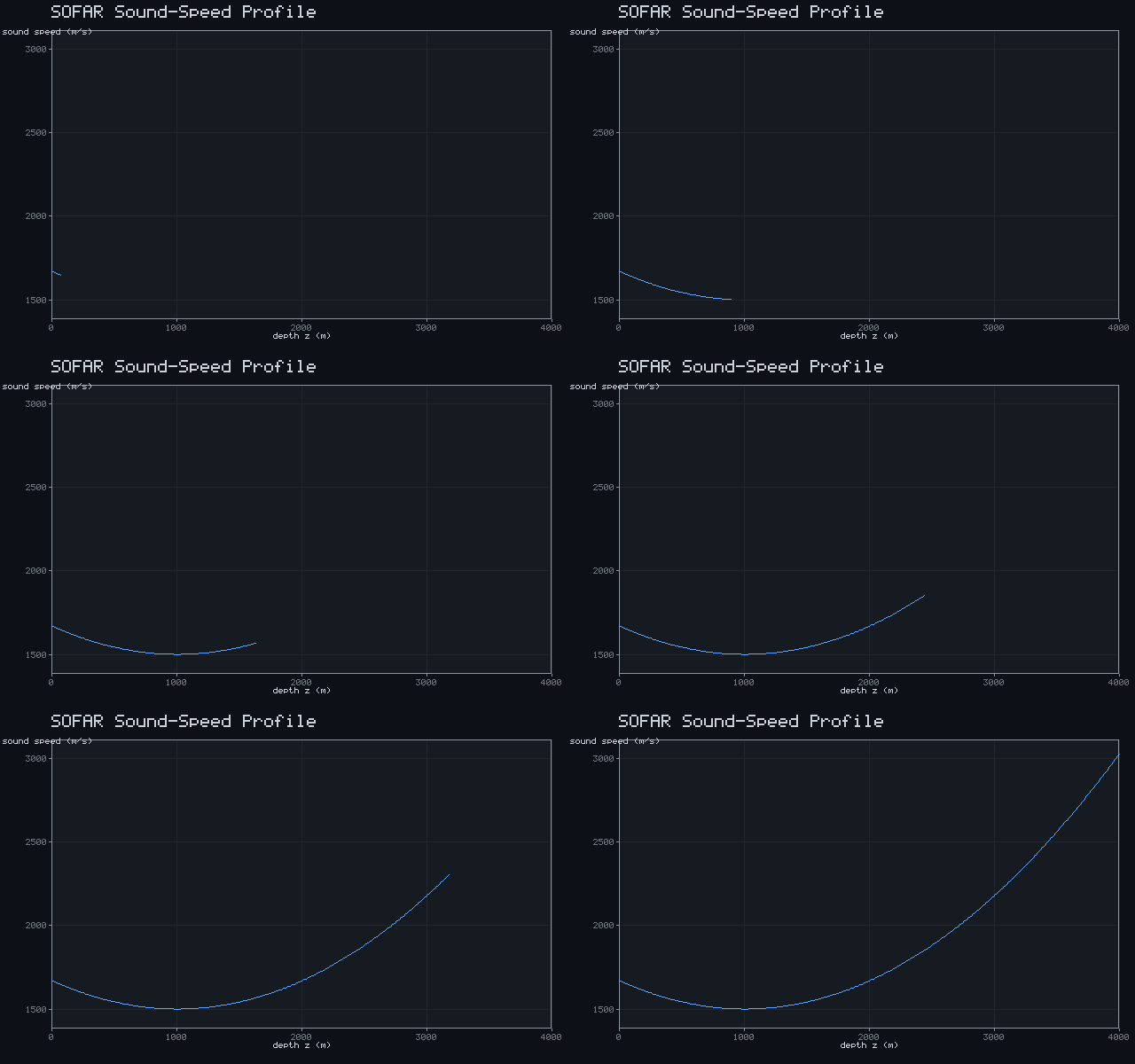

SOFAR Sound-Speed Profile

c = 1500 + 0.017(z−1000)²/100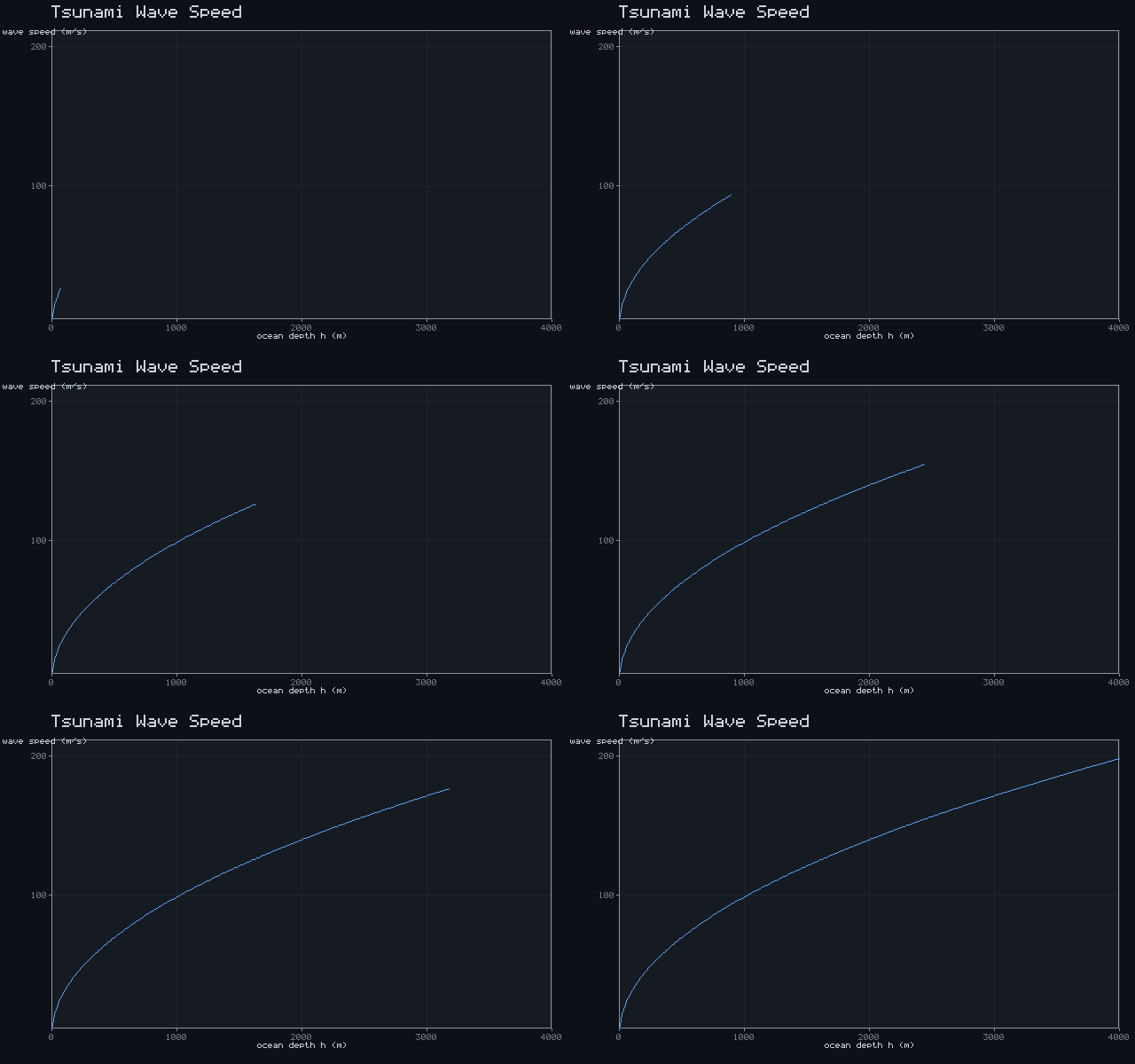

Tsunami Wave Speed

v = √(g·h)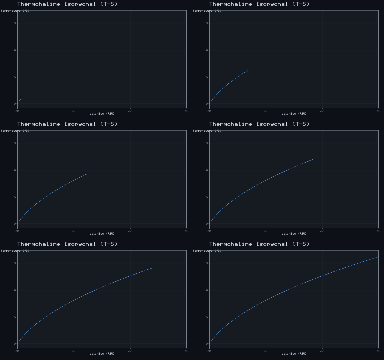

Thermohaline Isopycnal (T-S)

σ_t = 0.8(S−35) − 0.05T − 0.006T² = const

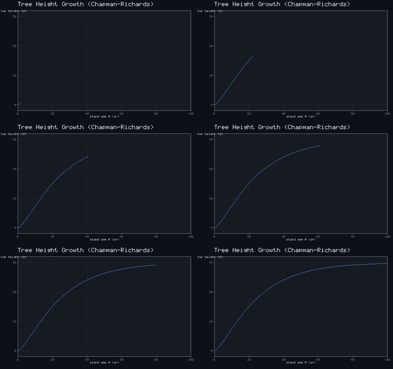
Tree Height Growth (Chapman-Richards)

H = 30(1 − e^(−0.05·A))^1.5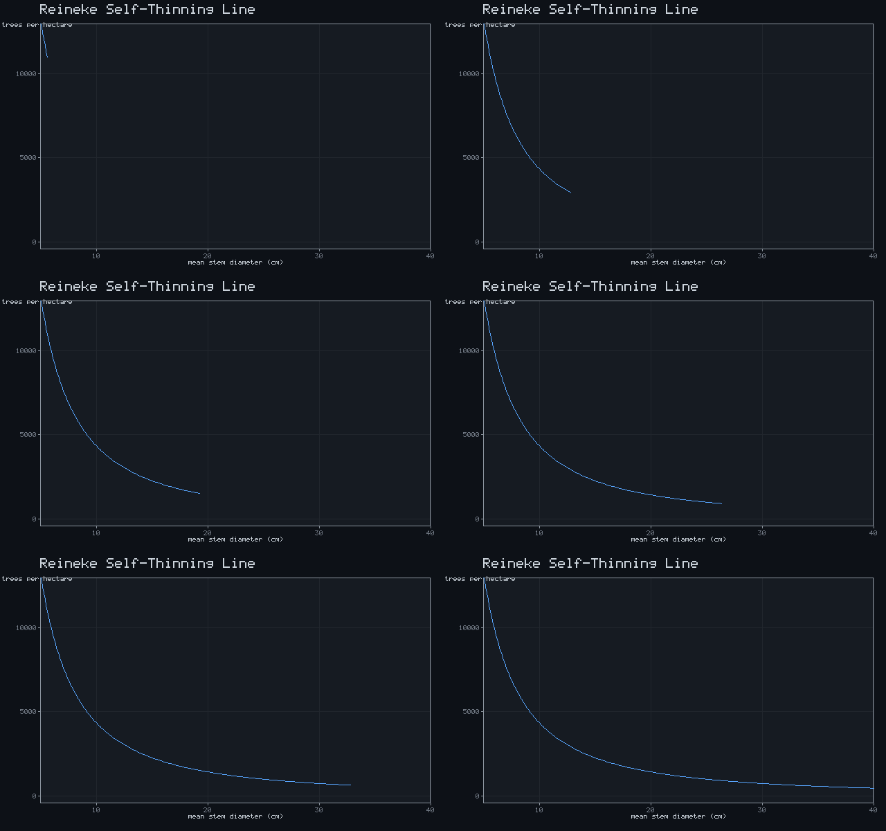

Reineke Self-Thinning Line

N = 1000(D/25)^(−1.605)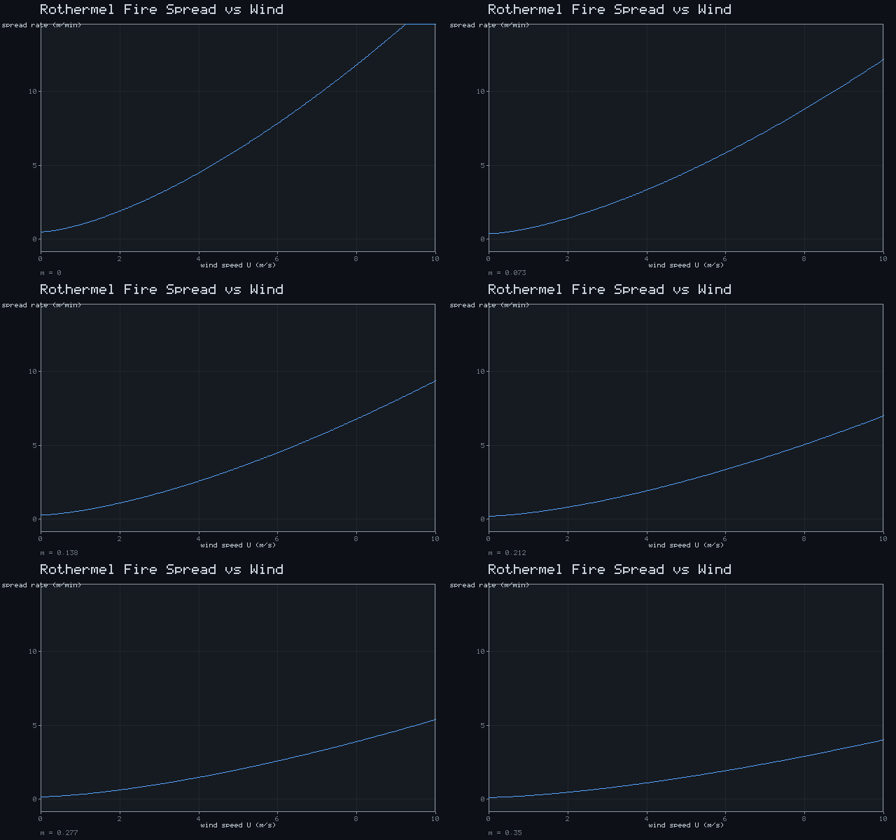

Rothermel Fire Spread vs Wind

R = R₀(1 + U^1.5)·e^(−k·M)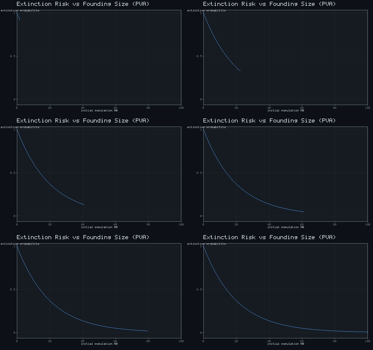

Extinction Risk vs Founding Size (PVA)

P_ext = e^(−N₀/N_c)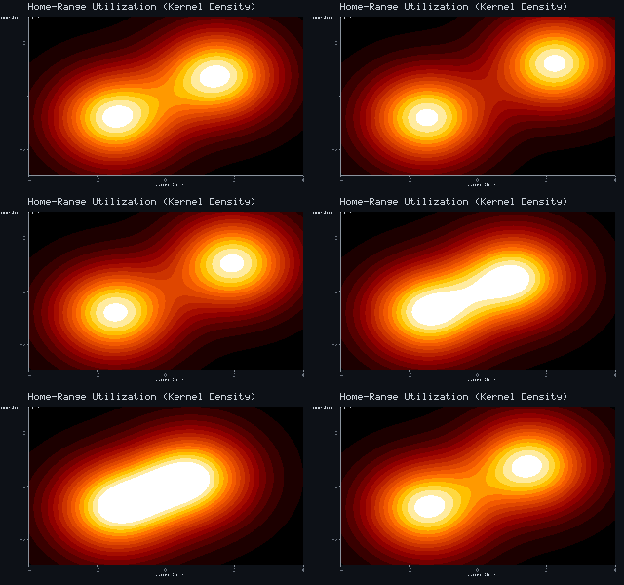

Home-Range Utilization (Kernel Density)

UD(x,y) = Σ e^(−rᵢ²/3)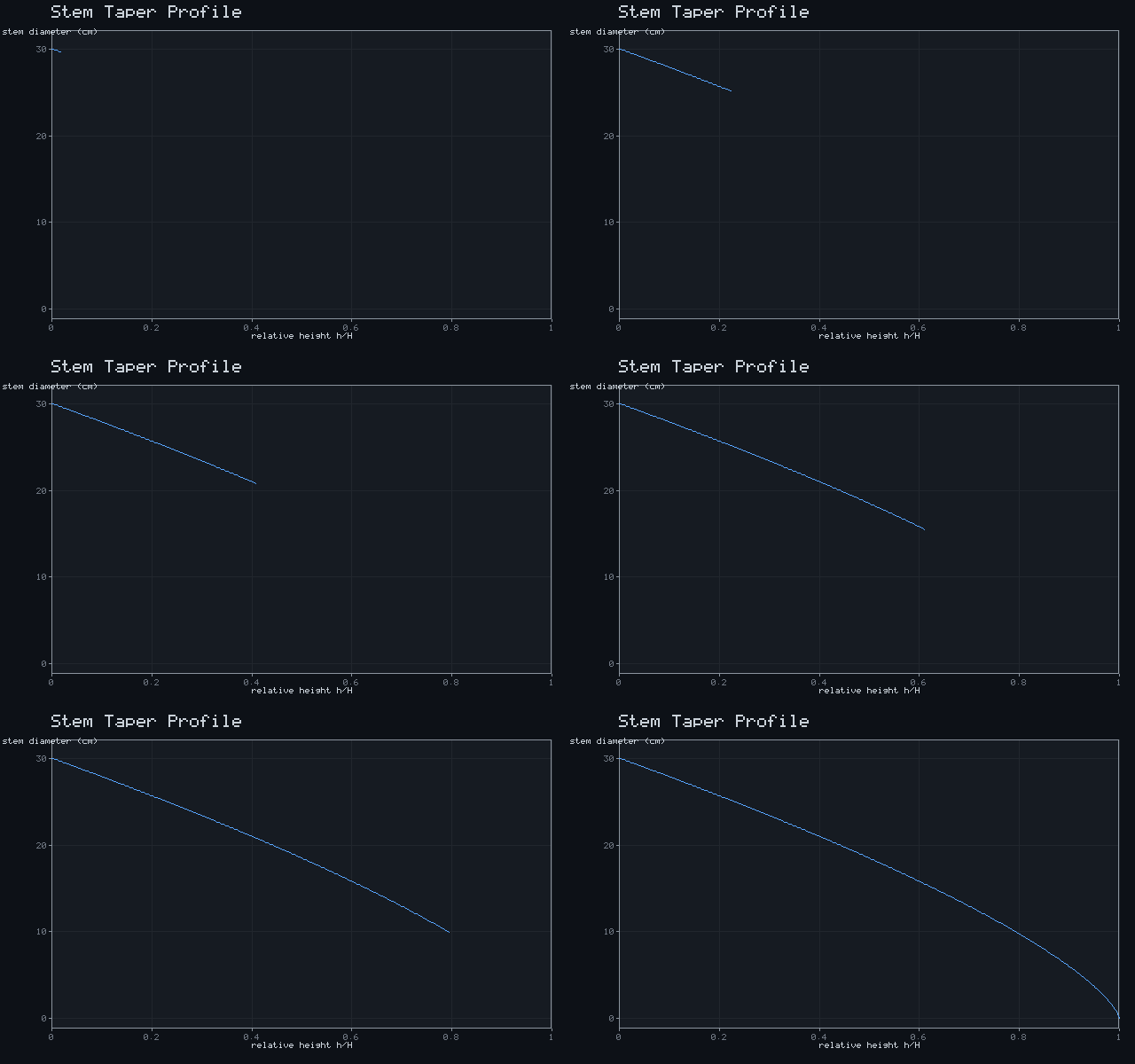

Stem Taper Profile

d = 30(1 − h/H)^0.7

Rising Smoke Plume

∂u/∂t + (u·∇)u = −∇p + ν∇²u (Navier-Stokes)

Smoke Blocked by a Glass Shelf

no-flow boundary at the solid barrier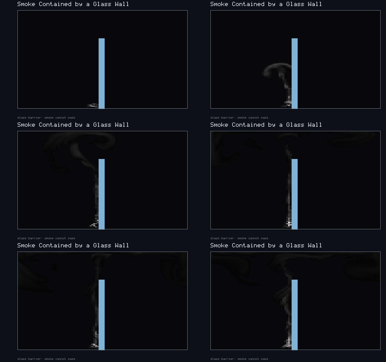

Smoke Contained by a Glass Wall

partition wall with an open top gap

Fire Plume

buoyancy ∝ temperature; hot gas rises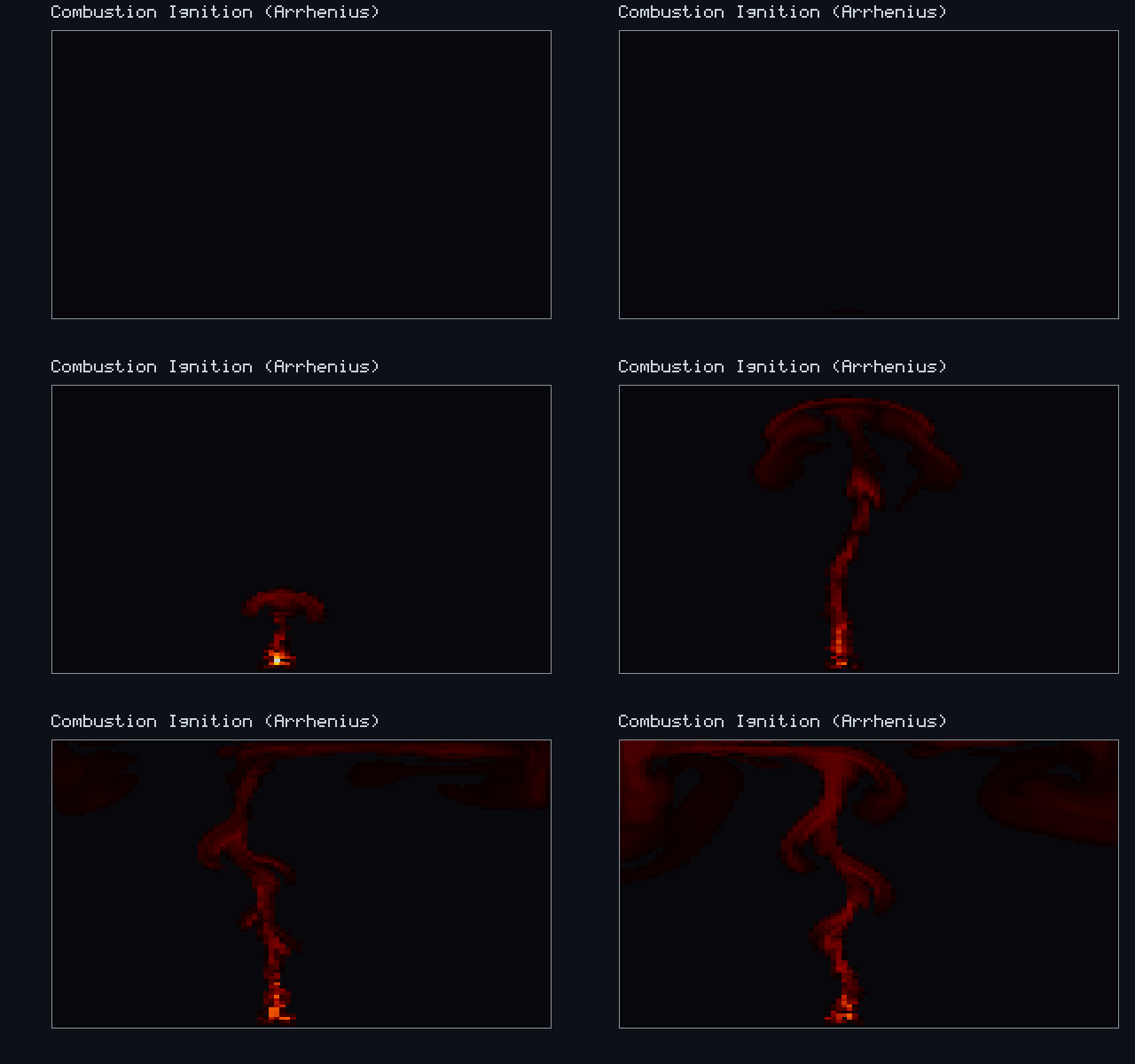

Combustion Ignition (Arrhenius)

k(T) = A·e^(−Eₐ/RT)

Rayleigh-Bénard Convection

heated floor + buoyancy → rolls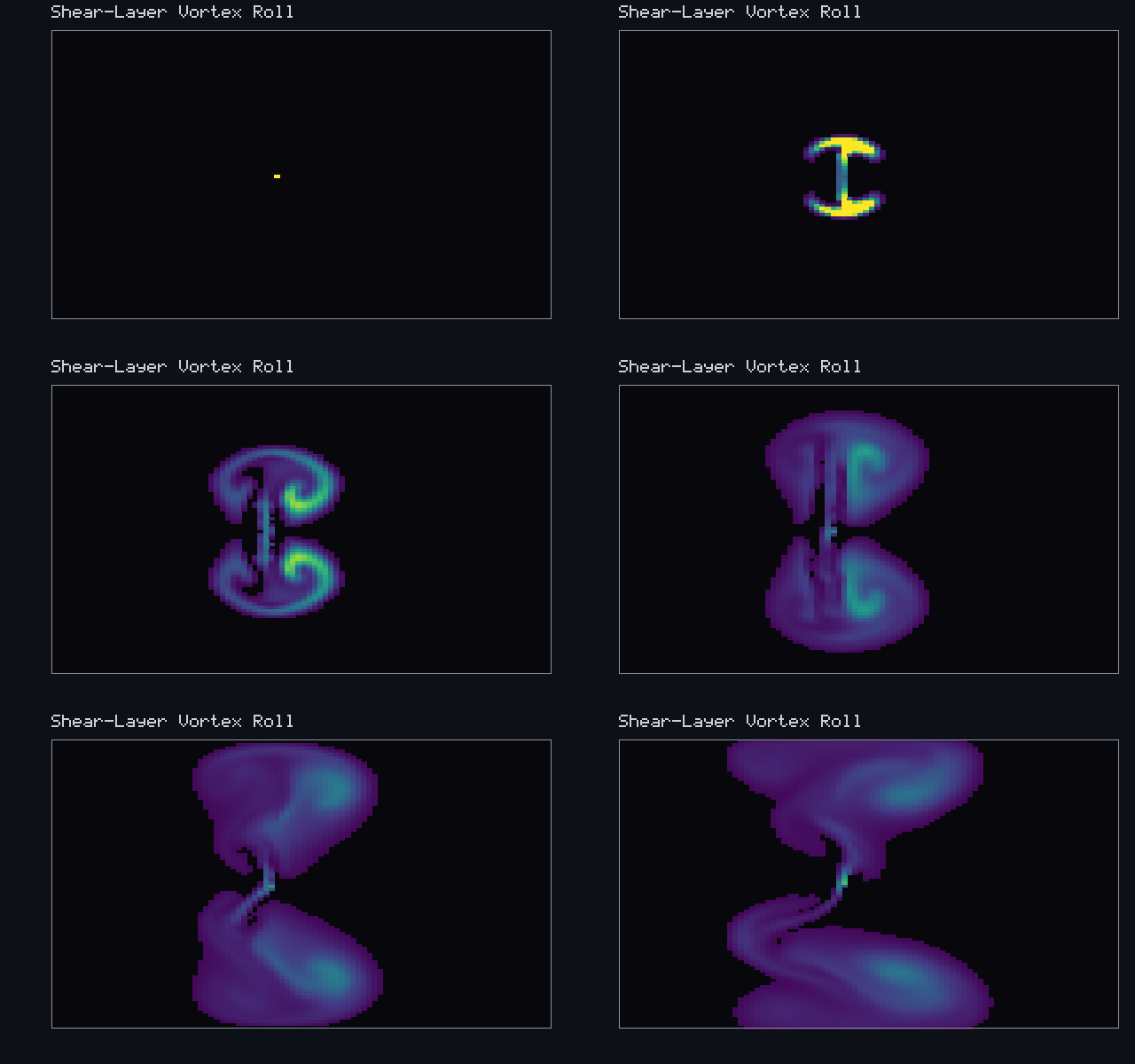

Shear-Layer Vortex Roll

Kelvin-Helmholtz shear instability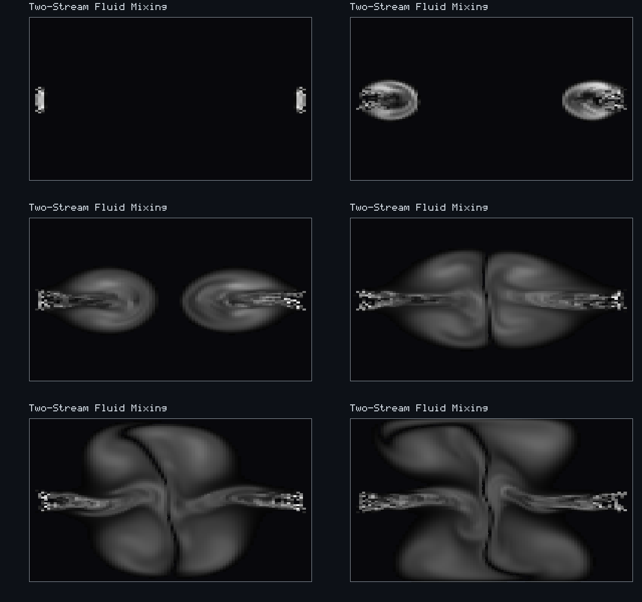

Two-Stream Fluid Mixing

advection-diffusion of two streams

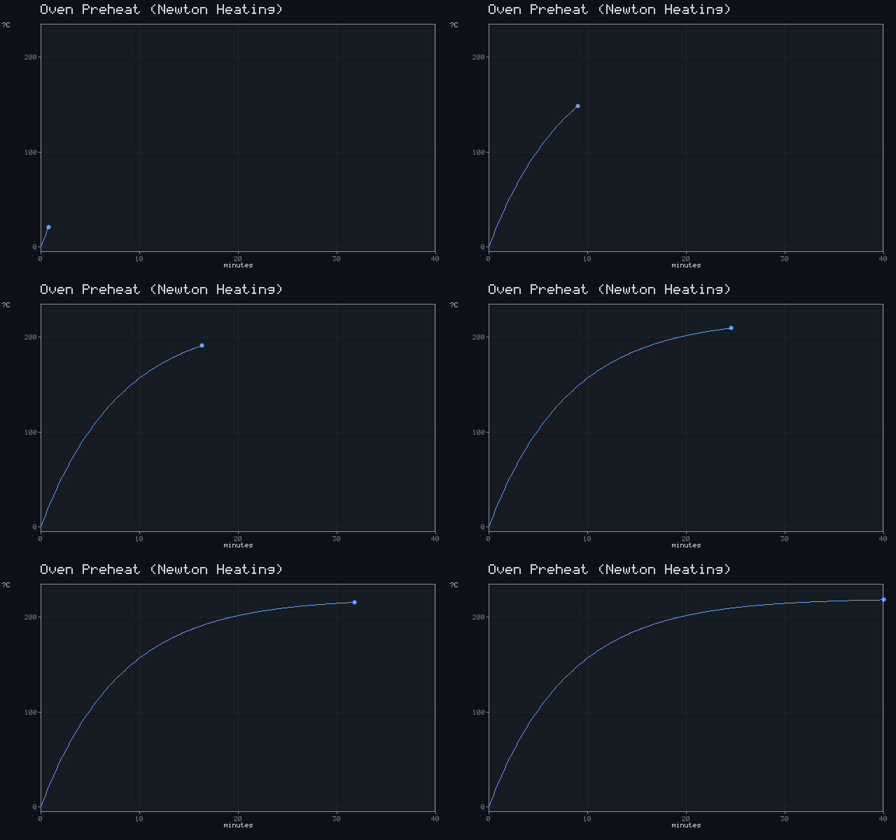
Oven Preheat (Newton Heating)

T(t) = T_set·(1 − e^(−t/τ))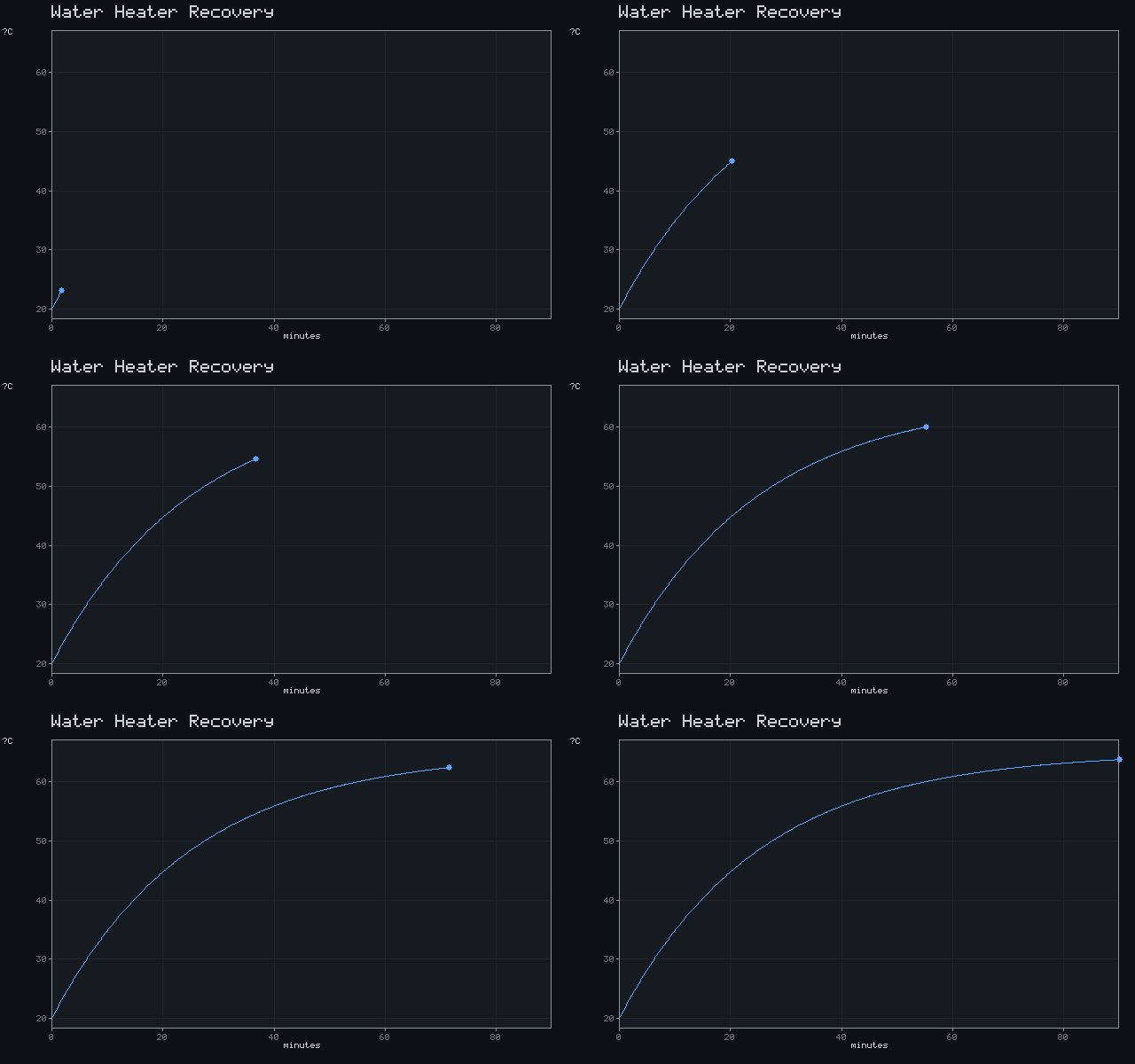

Water Heater Recovery

T(t) = T_in + ΔT·(1 − e^(−t/τ))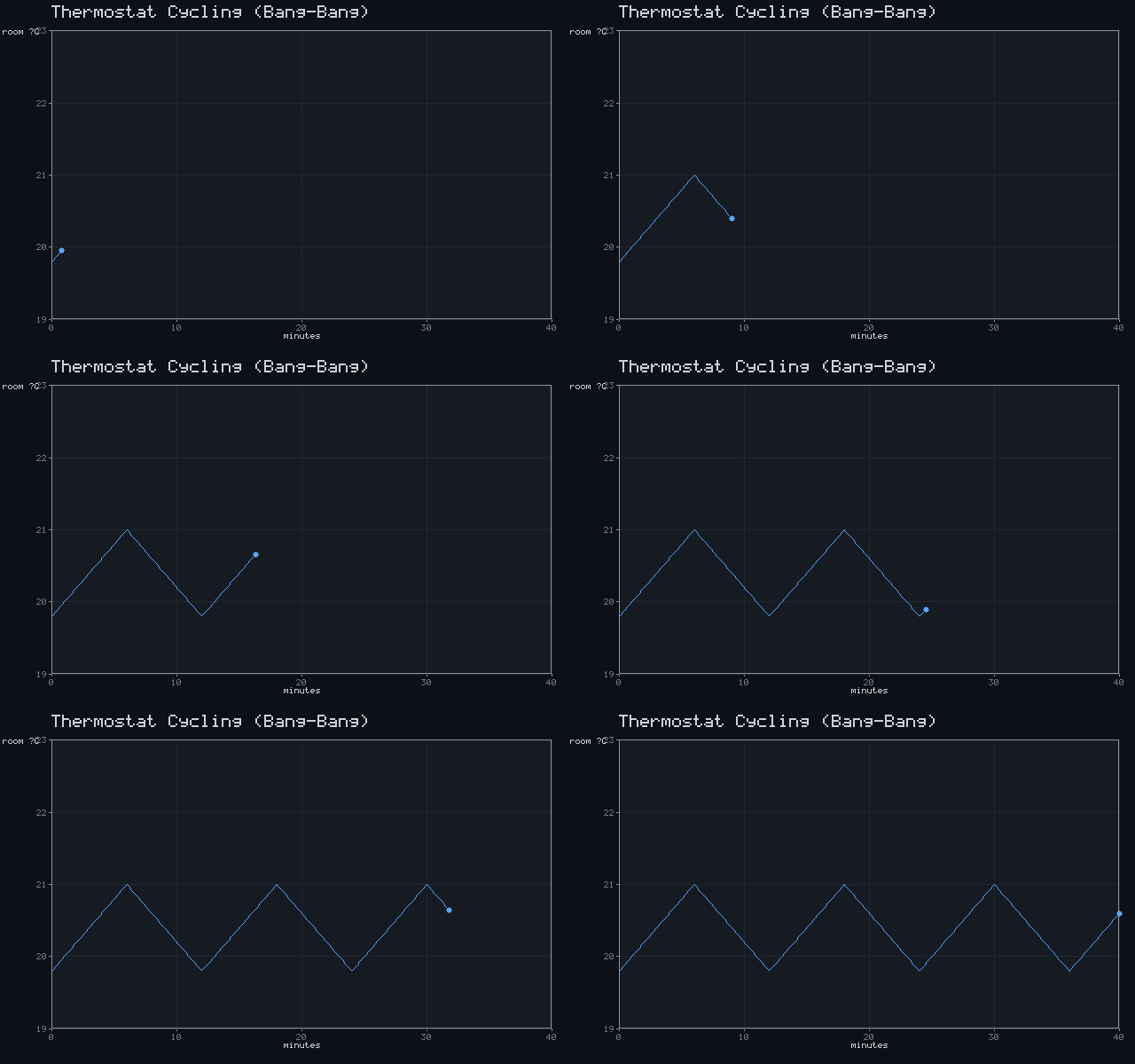

Thermostat Cycling (Bang-Bang)

furnace on below setpoint, off above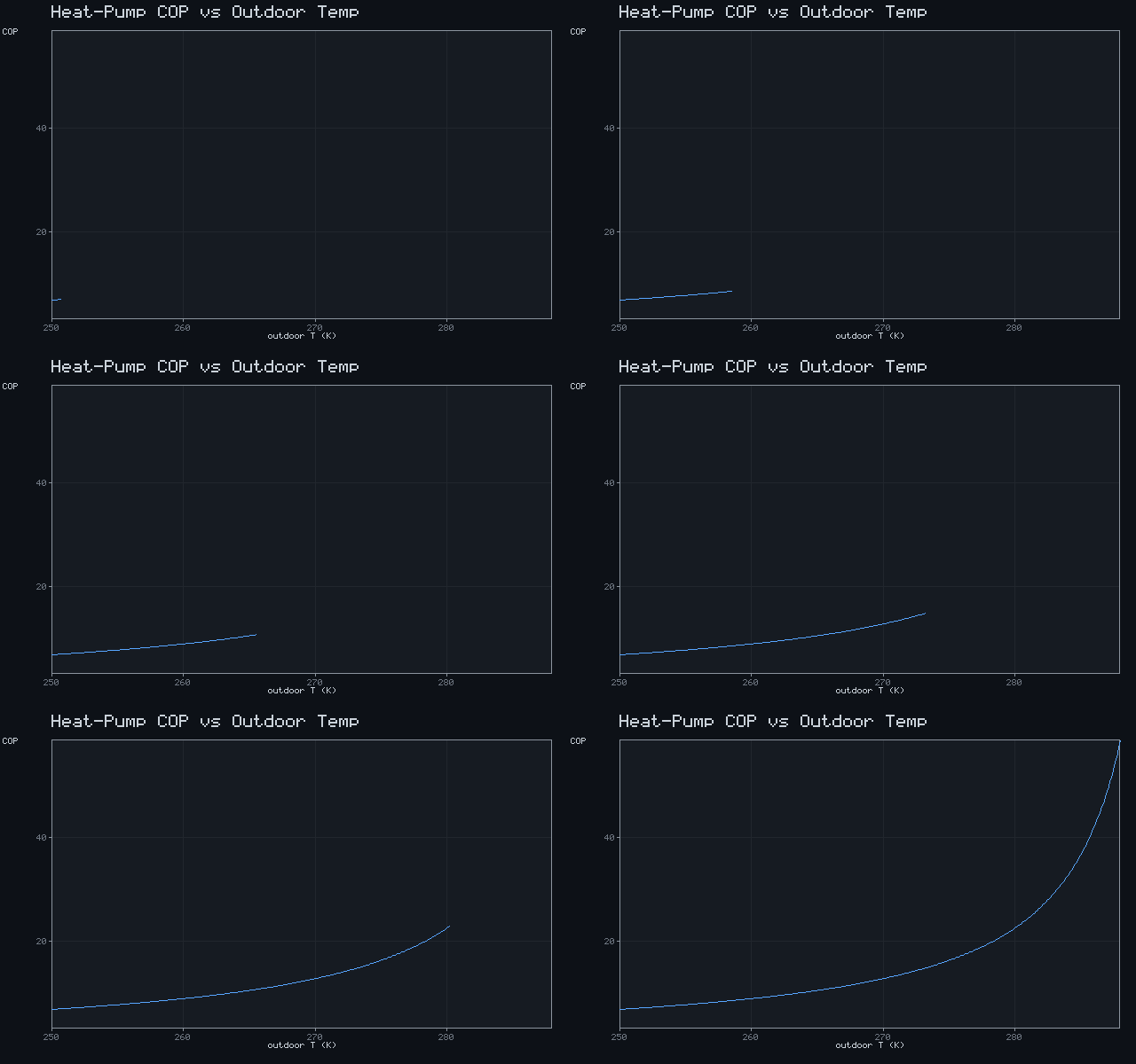

Heat-Pump COP vs Outdoor Temp

COP = T_h / (T_h − T_c)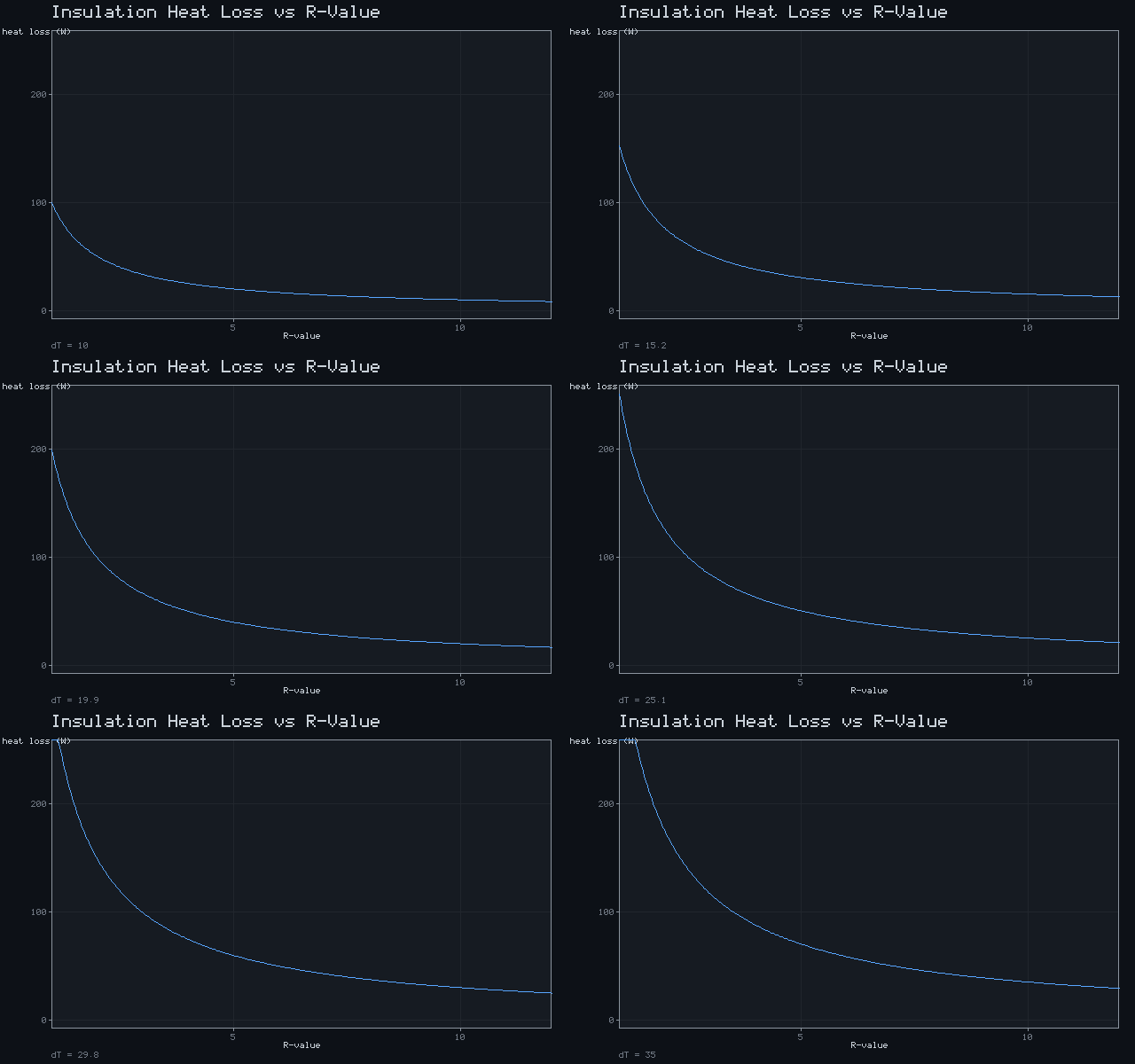

Insulation Heat Loss vs R-Value

Q = A·ΔT / R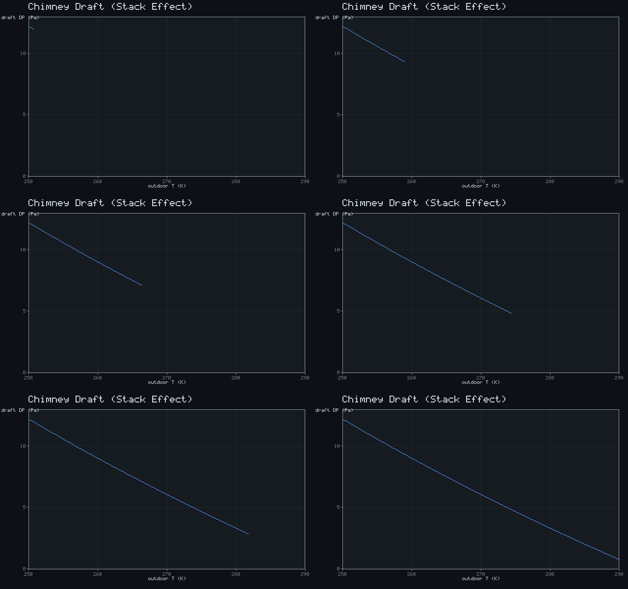

Chimney Draft (Stack Effect)

ΔP = C·h·(1/T_out − 1/T_in)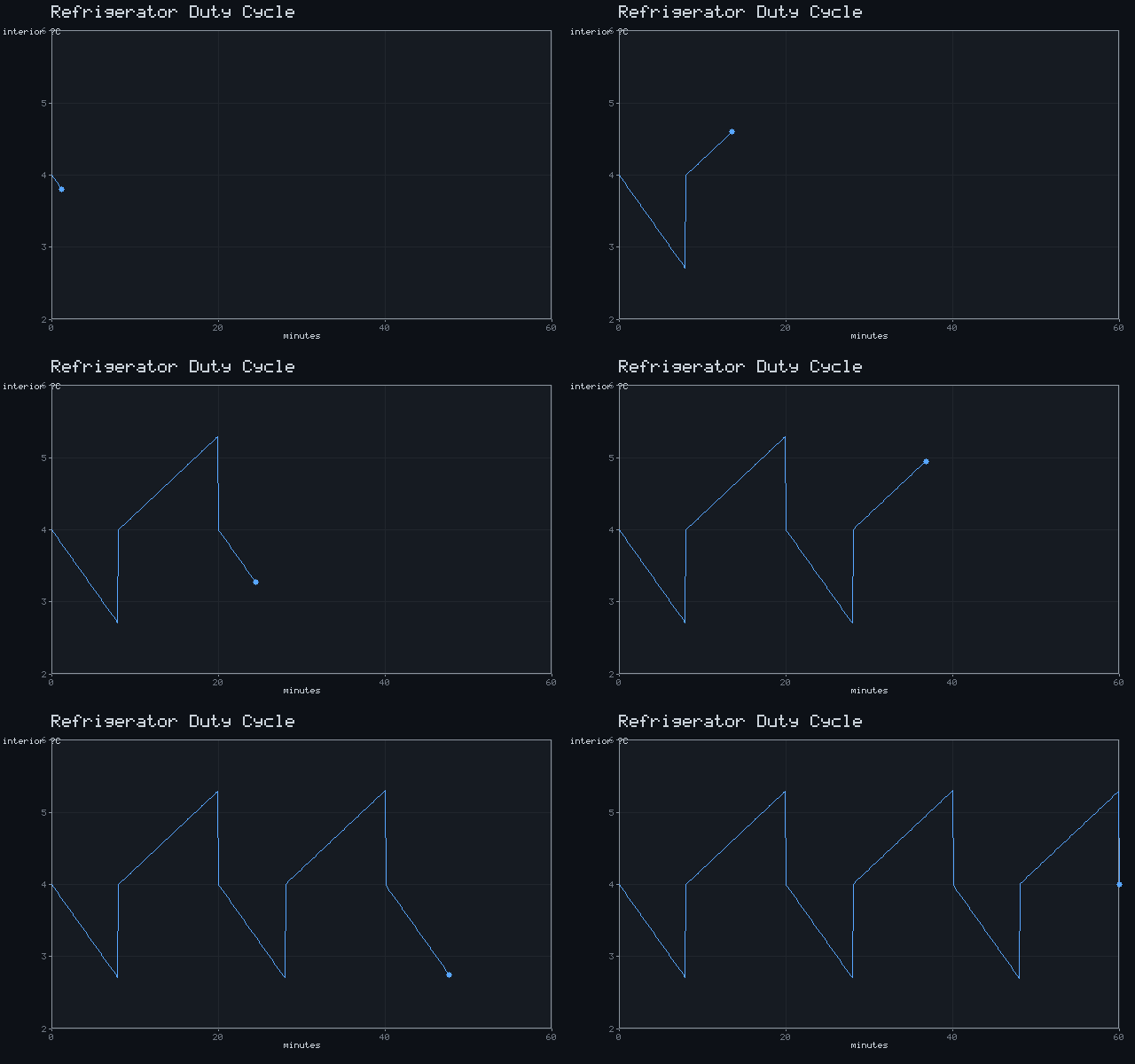

Refrigerator Duty Cycle

compressor cycles about the setpoint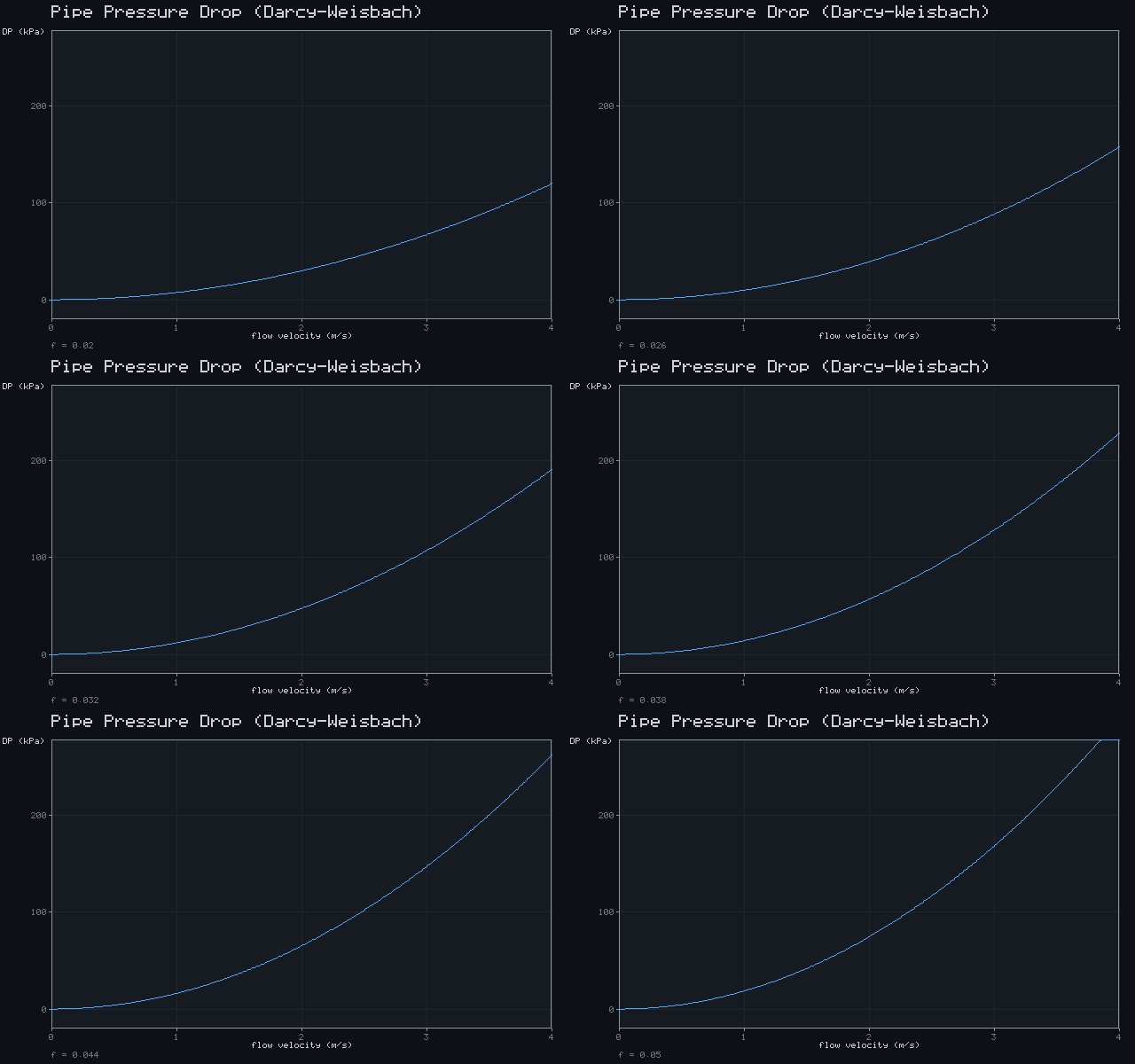

Pipe Pressure Drop (Darcy-Weisbach)

ΔP = f·(L/D)·(ρv²/2)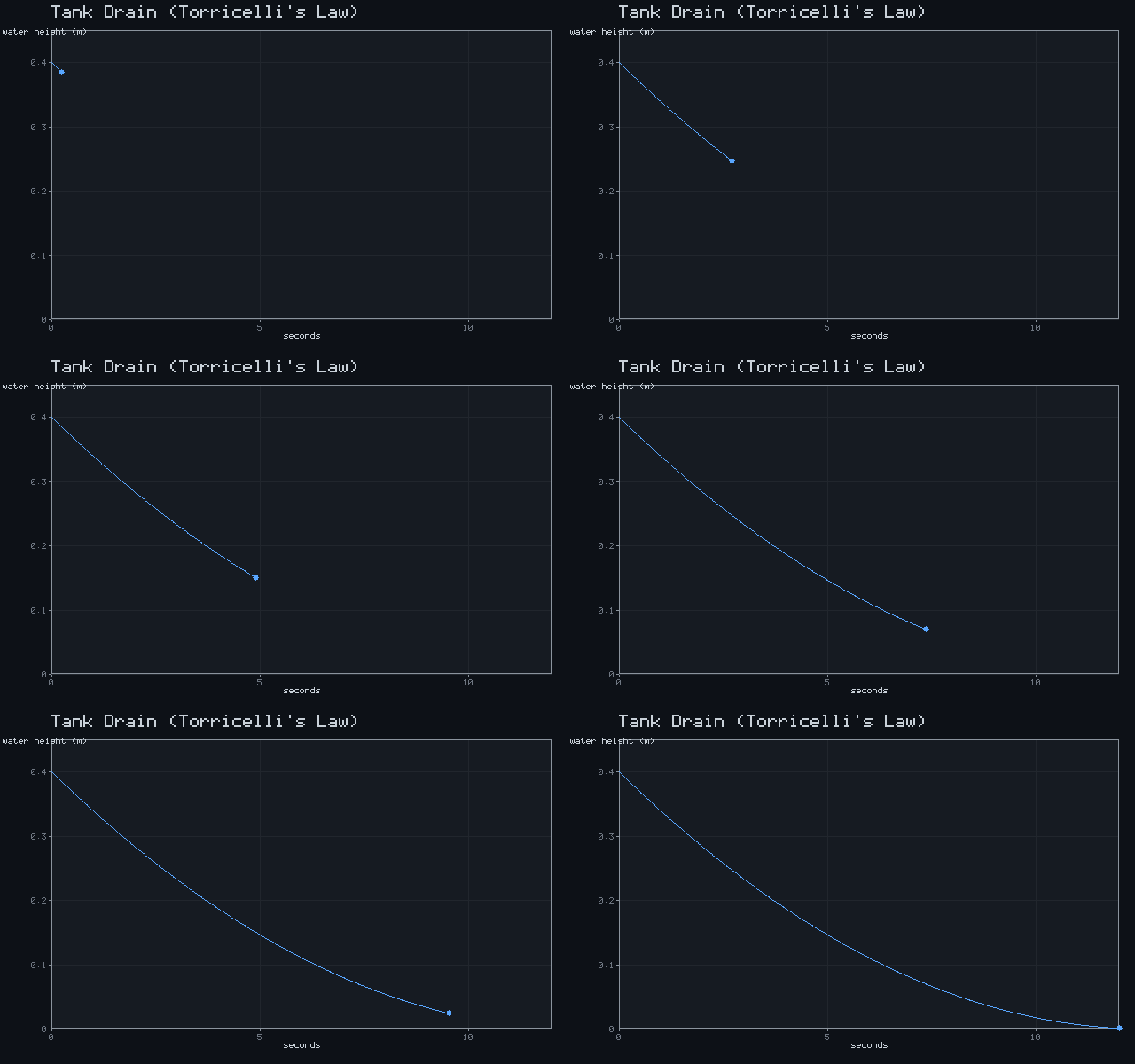

Tank Drain (Torricelli's Law)

h(t) = (√h₀ − k t)² · v = √(2gh)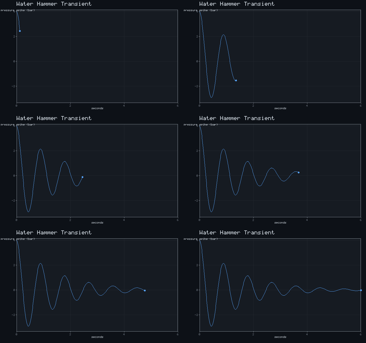

Water Hammer Transient

ΔP surge, then damped oscillation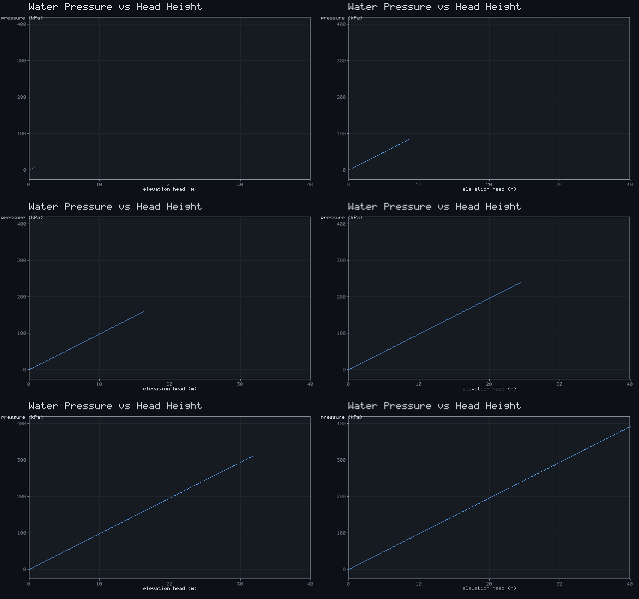

Water Pressure vs Head Height

P = ρ g h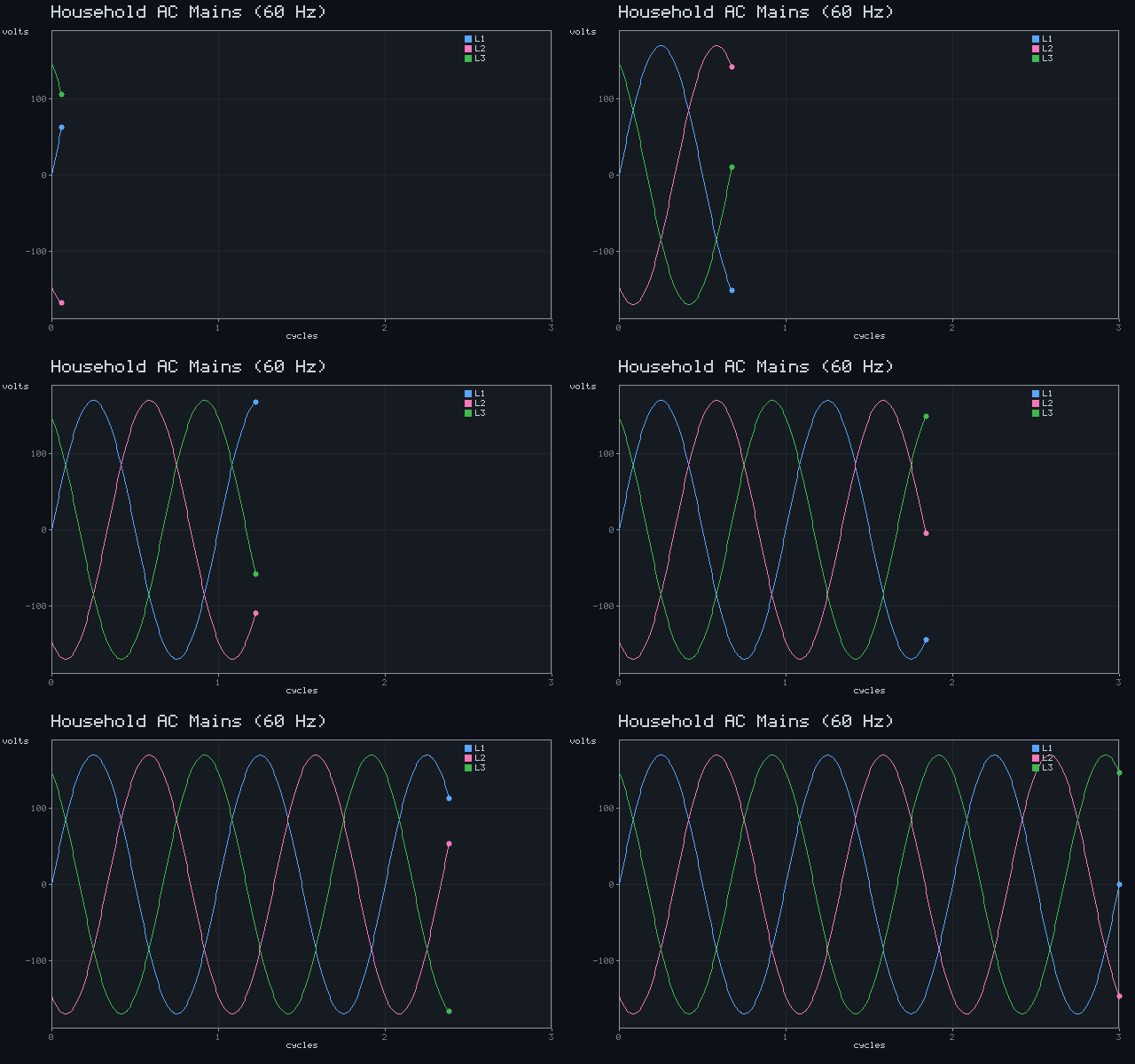

Household AC Mains (60 Hz)

v(t) = 170·sin(2π·60·t), V_rms = 120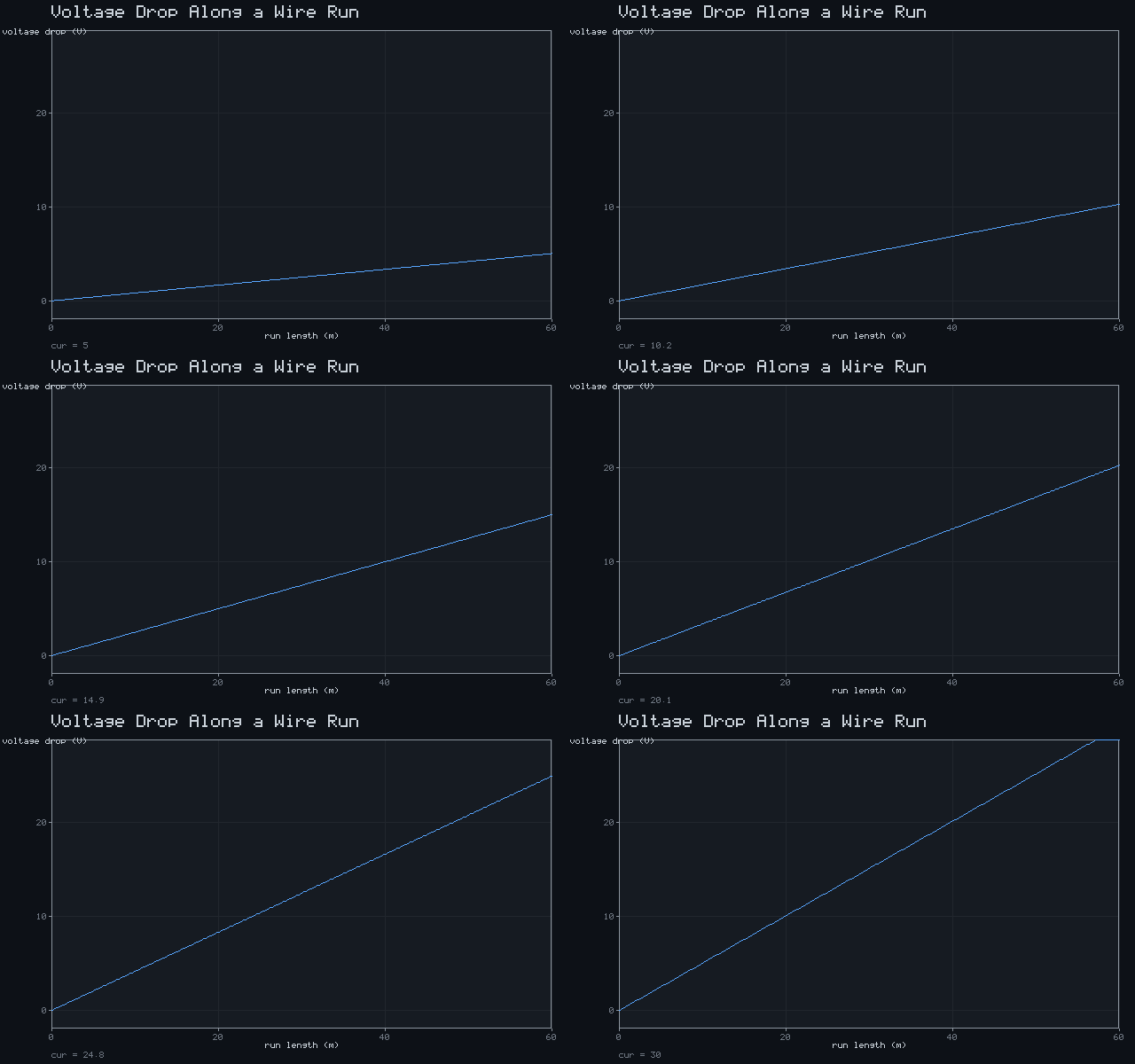

Voltage Drop Along a Wire Run

V_drop = I·ρ·2L / A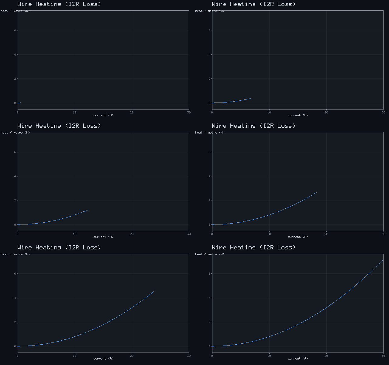

Wire Heating (I²R Loss)

P = I²R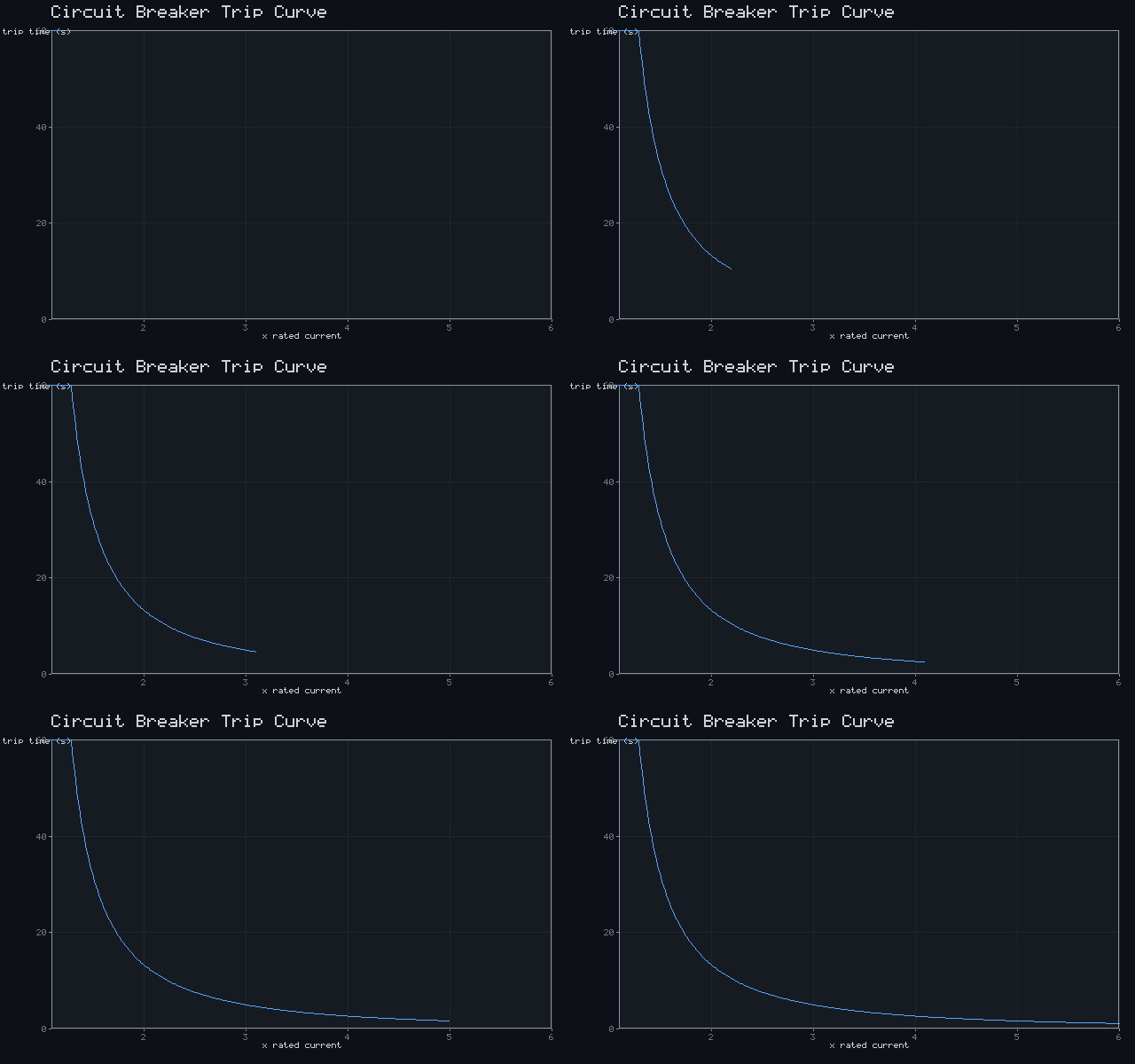

Circuit Breaker Trip Curve

t_trip ∝ 1/(I/I_rated)² (inverse-time)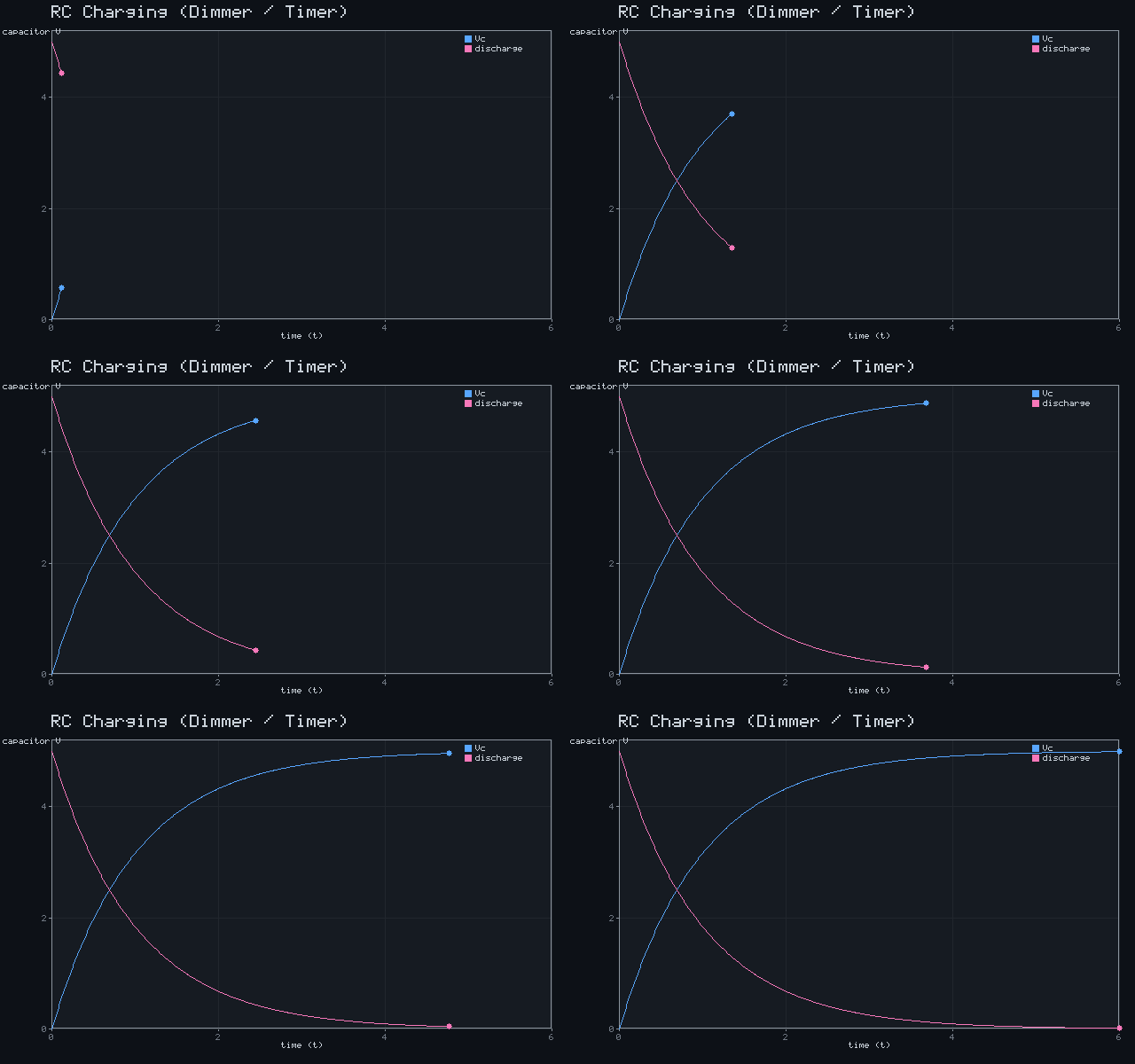

RC Charging (Dimmer / Timer)

V_c = V·(1 − e^(−t/RC))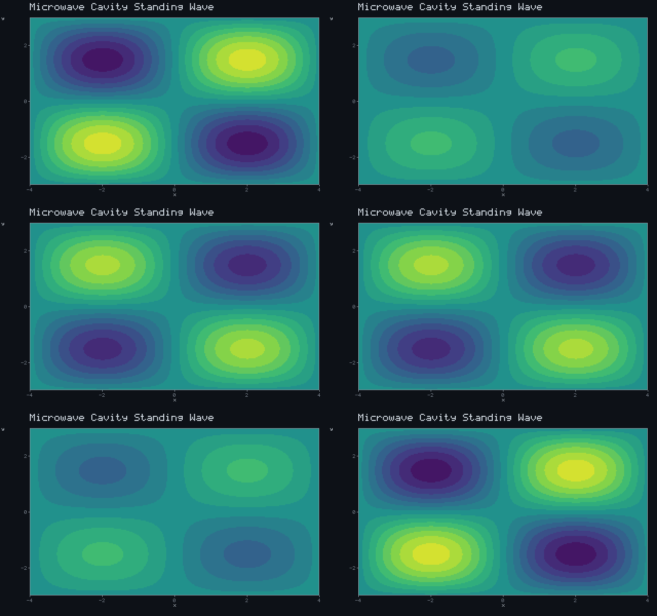

Microwave Cavity Standing Wave

E(x,y) = sin(mπx/a)·sin(nπy/b)·cos ωt @ 2.45 GHz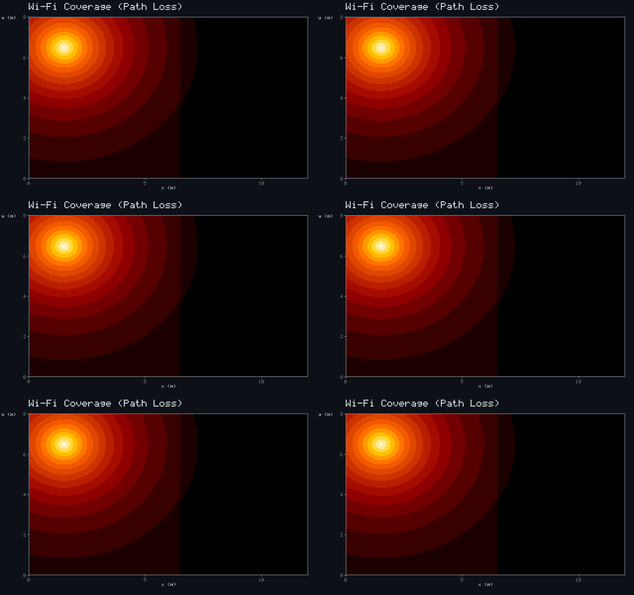

Wi-Fi Coverage (Path Loss)

P ∝ 1/r² with wall attenuation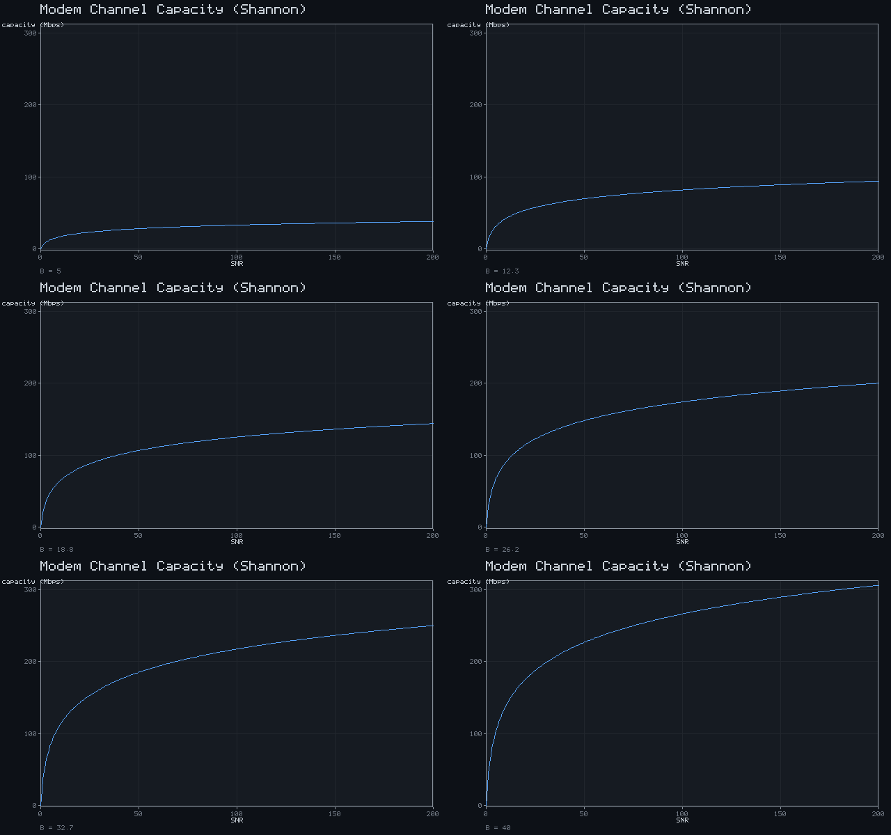

Modem Channel Capacity (Shannon)

C = B·log₂(1 + SNR)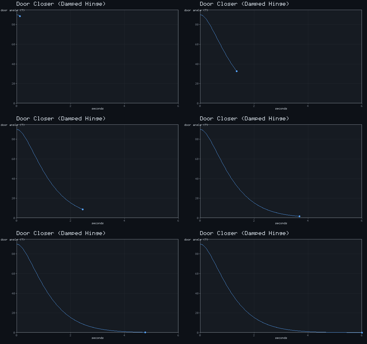

Door Closer (Damped Hinge)

critically damped: θ = θ₀(1+βt)e^(−βt)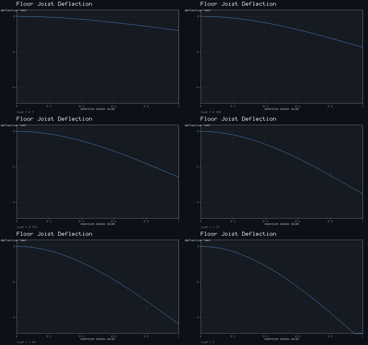

Floor Joist Deflection

y(x) = w·x²(3L − x)/6EI

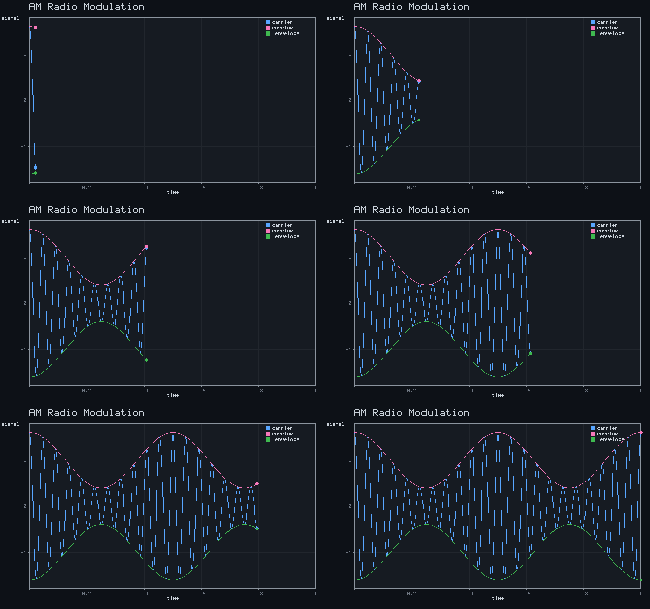
AM Radio Modulation

v(t) = (1 + m·cos ω_m t)·cos ω_c t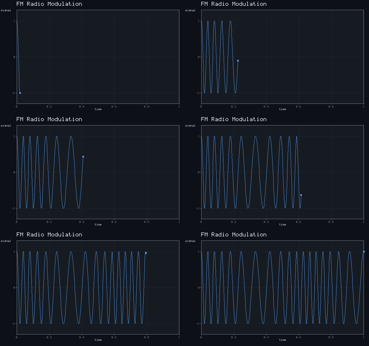

FM Radio Modulation

v(t) = cos(ω_c t + β·sin ω_m t)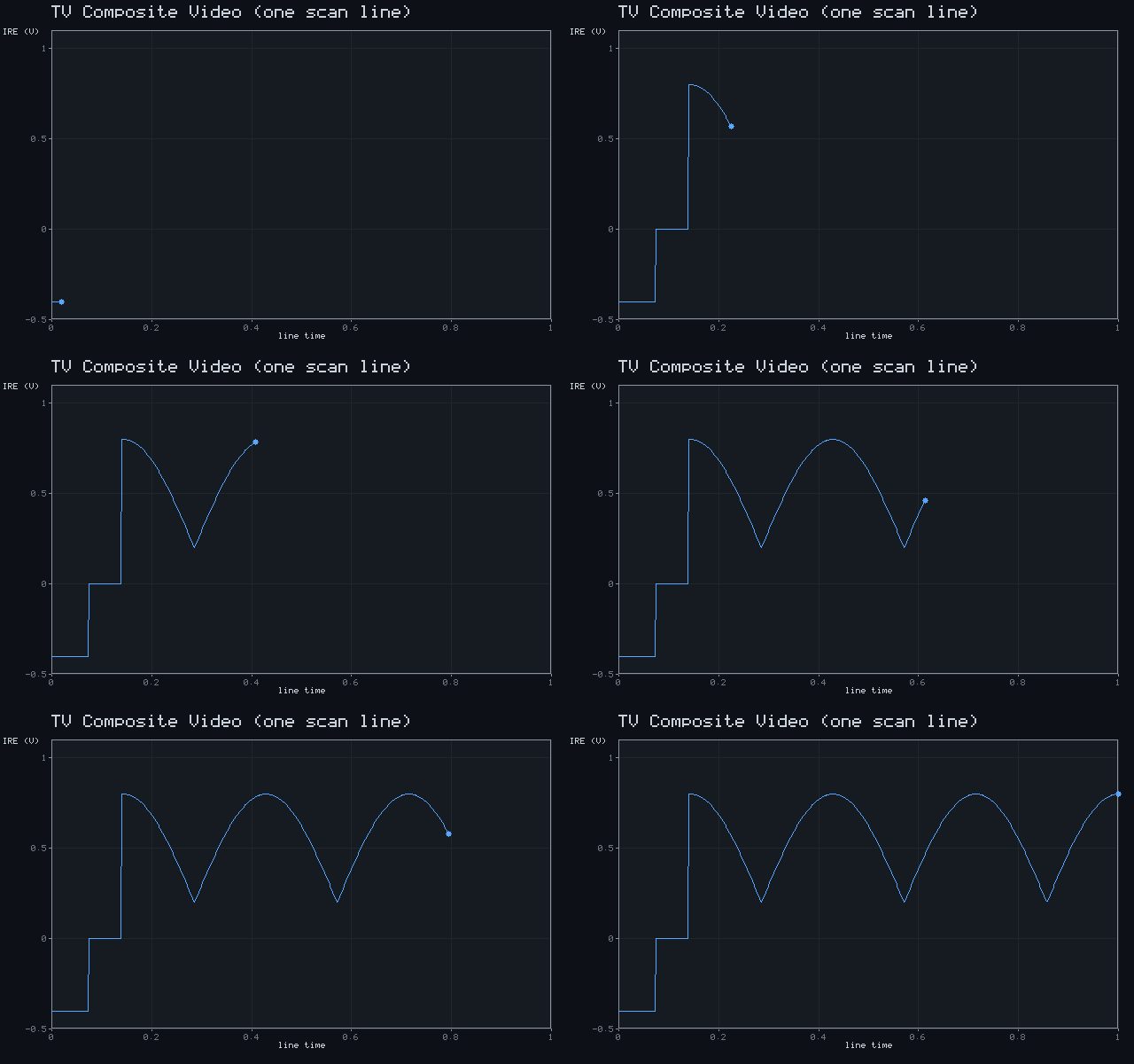

TV Composite Video (one scan line)

sync tip → back porch → active luminance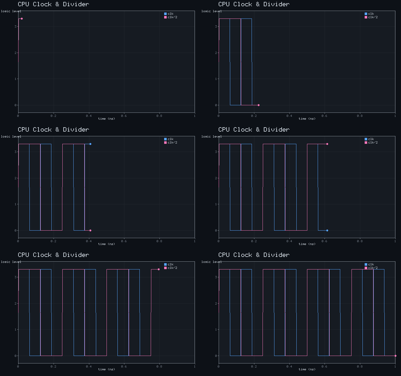

CPU Clock & Divider

square wave + ÷2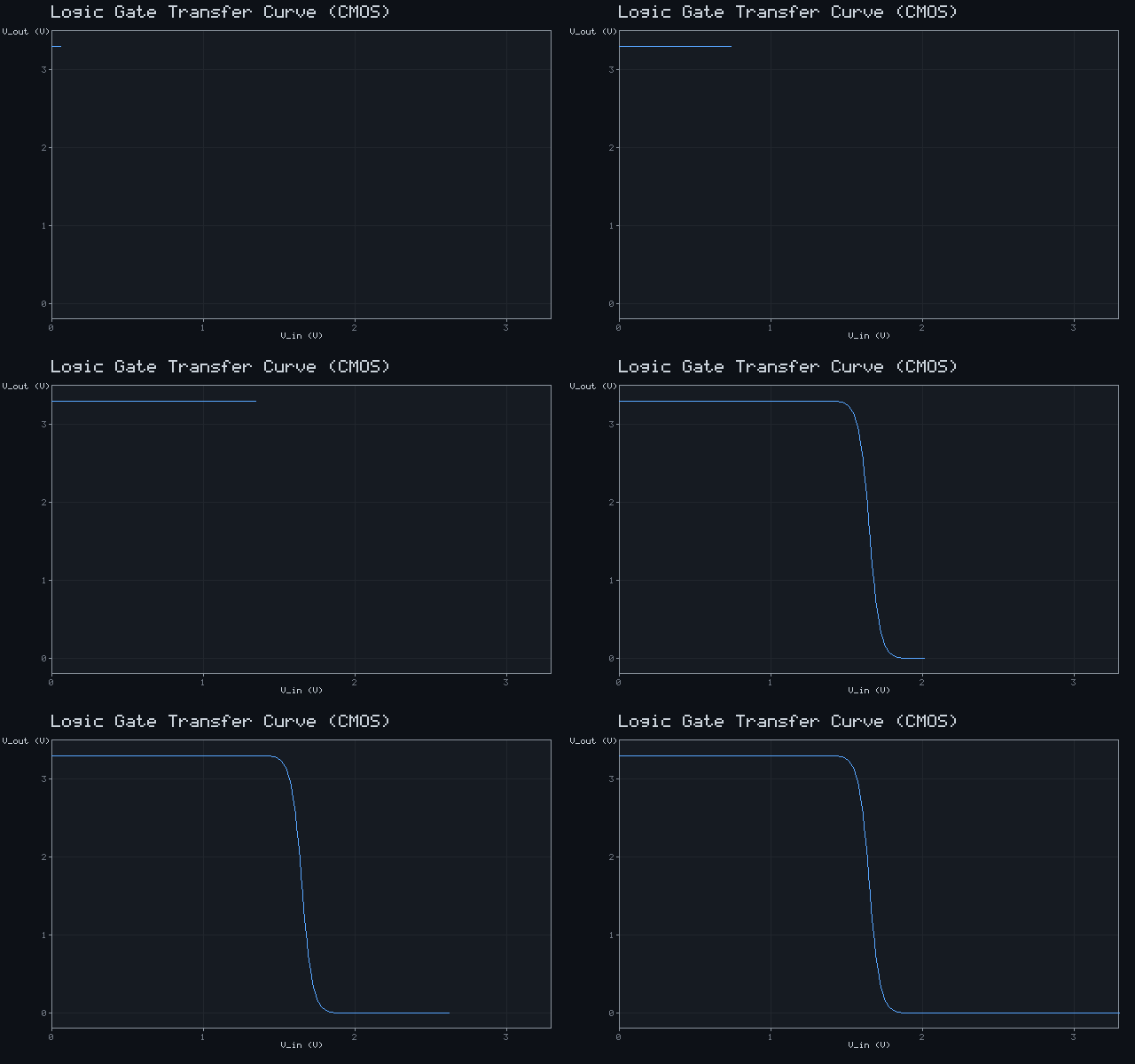

Logic Gate Transfer Curve (CMOS)

V_out sharply flips at V_DD/2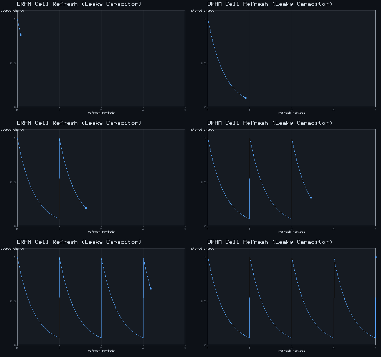

DRAM Cell Refresh (Leaky Capacitor)

V = V₀·e^(−t/τ), refreshed each period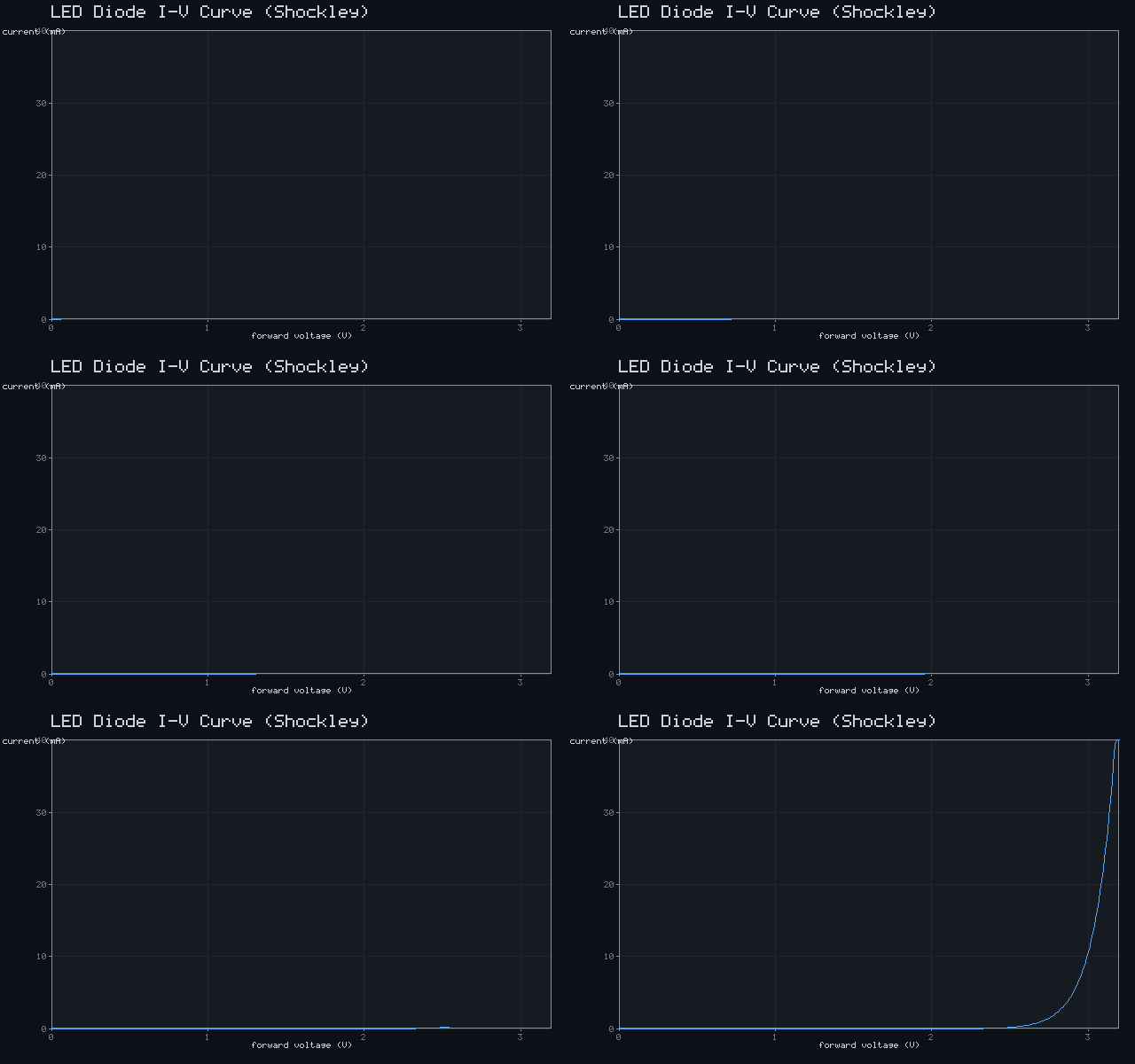

LED Diode I-V Curve (Shockley)

I = I_s·(e^(V/nV_T) − 1)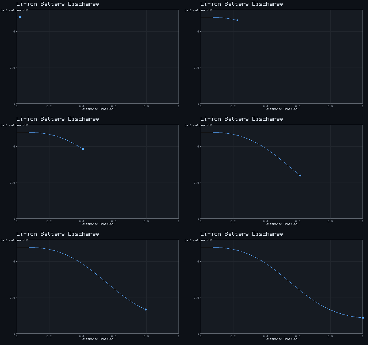

Li-ion Battery Discharge

terminal voltage vs state of charge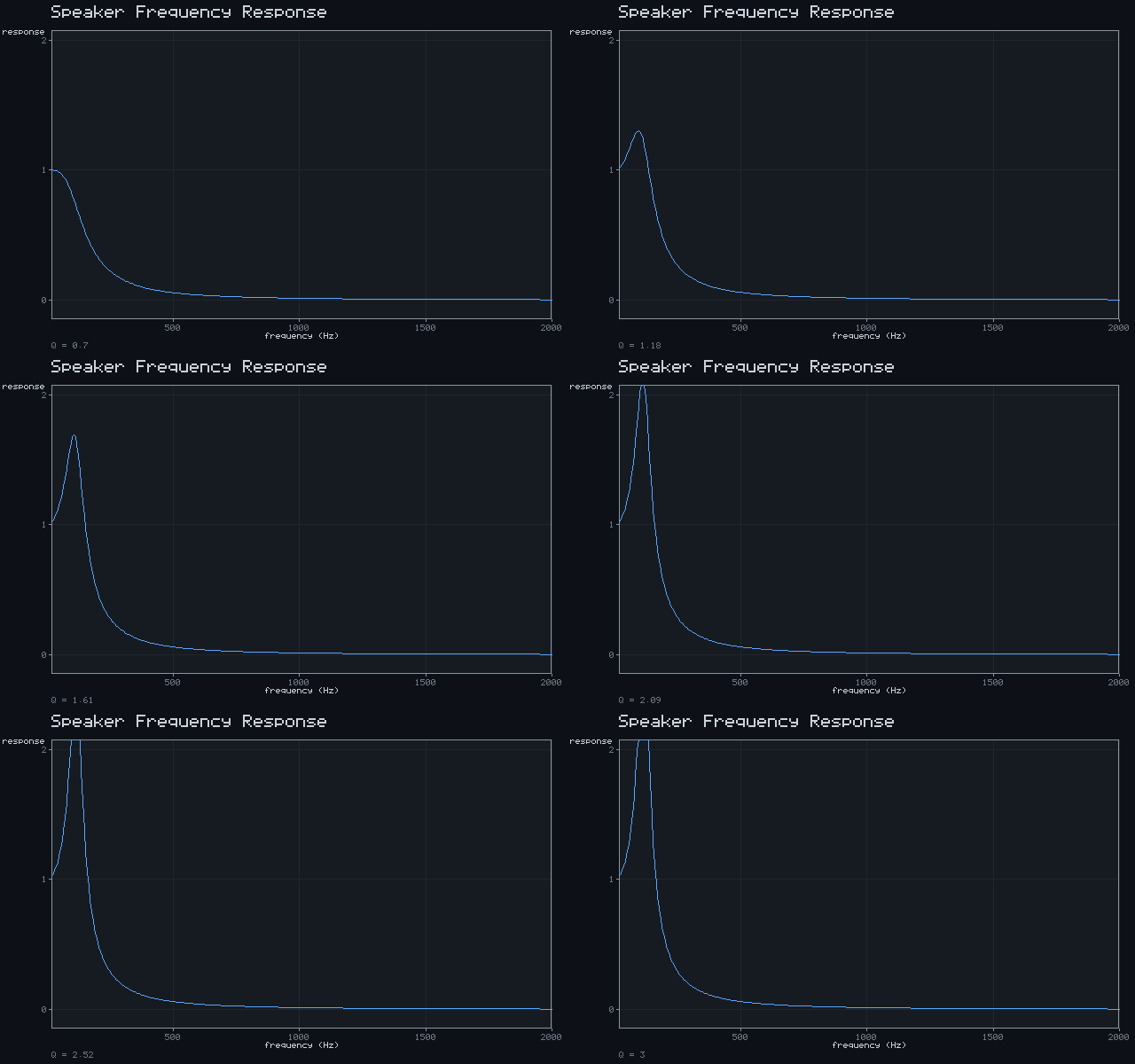

Speaker Frequency Response

|H(f)| = 1/√((1−(f/f₀)²)² + (f/Qf₀)²)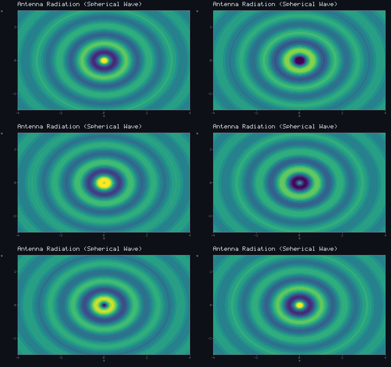

Antenna Radiation (Spherical Wave)

E = cos(kr − ωt)/r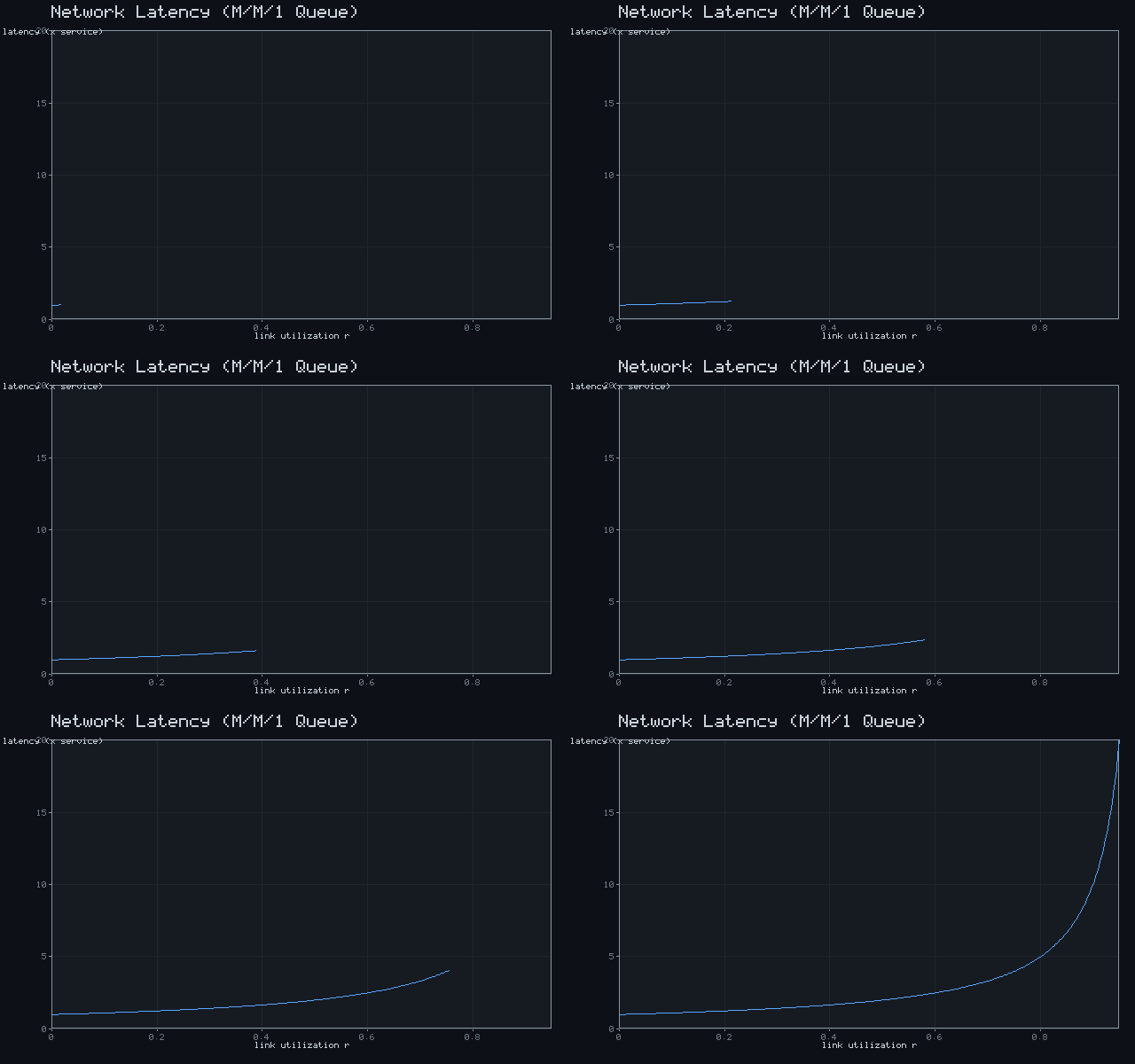

Network Latency (M/M/1 Queue)

W = 1/(μ − λ) → ∞ as ρ → 1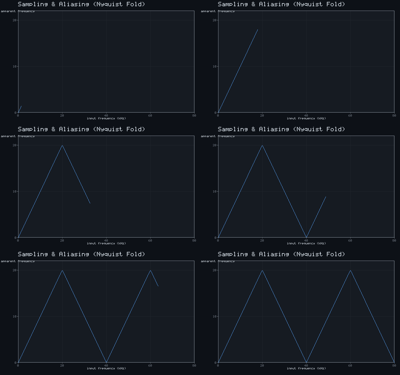

Sampling & Aliasing (Nyquist Fold)

f_alias = |f − f_s·round(f/f_s)|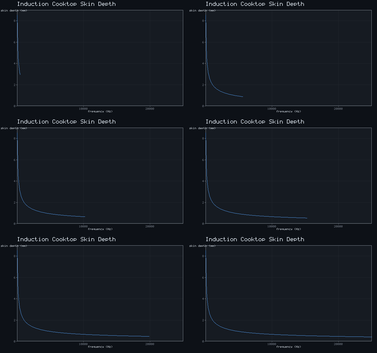

Induction Cooktop Skin Depth

δ = 1/√(πfμσ)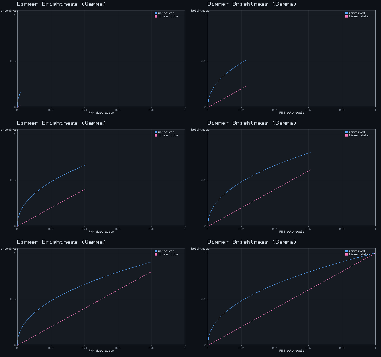

Dimmer Brightness (Gamma)

perceived ≈ duty^(1/2.2)